文章目录
0 库函数
import pandas as pd
1 原始数据检视
df_train = pd.read_csv(r'C:\Users\chen\Desktop\leetcode\kaggle\房价预测\train.csv')
df_test = pd.read_csv(r'C:\Users\chen\Desktop\leetcode\kaggle\房价预测\test.csv')

pd.set_option('max_columns', 10000)      # 控制显示的列范围,查看数据的时候,显示所有数据,而且数据表中没有省略号
pd.set_option('max_rows', 500)
df_train.head()
df_train.info()                      # 查看训练集基本信息,如下图
display(df_train.shape)              # 查看训练集数据的维度
2 数据的探索性可视化分析
使用pandas_profiling模块工具一键生成探索性数据分析报告。
ppf.ProfileReport(df_train) # 一键进行探索性可视化分析
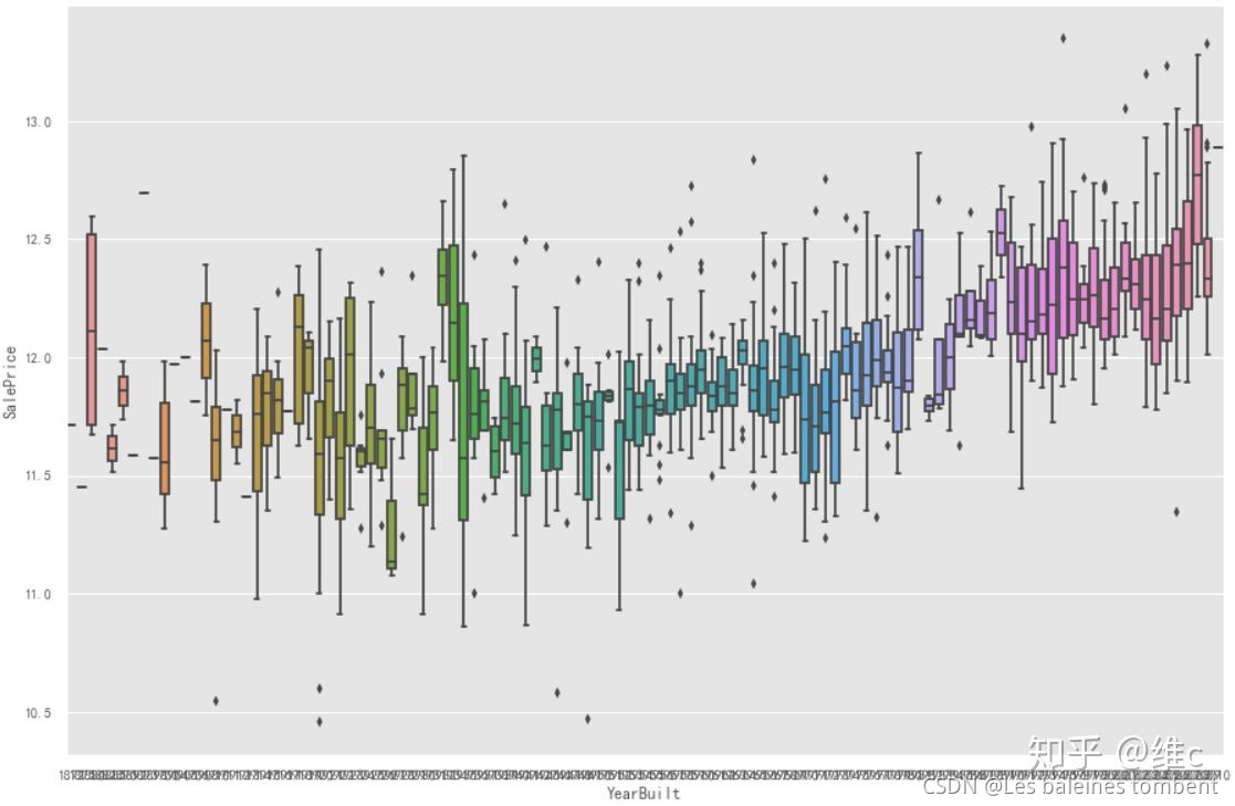
2.1 绘制箱线图,查看异常值分布情况
plt.figure(figsize=(15,12))
sns.boxplot(df_train.YearBuilt, df_train.SalePrice)##箱型图是看异常值的,离群点
plt.show()
3 数据清洗
3.1 异常值处理
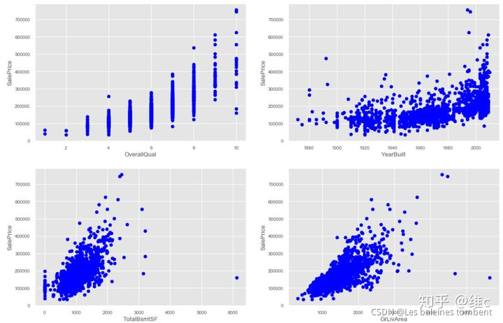
那么根据这四个变量和目标值之间的关系绘制散点图检查异常值点:
plt.figure(figsize=(18,12))

plt.subplot(2, 2, 1)
plt.scatter(x=df_train.OverallQual, y=df_train.SalePrice,color='b') ##可以用来观察存在线型的关系
plt.xlabel("OverallQual", fontsize=13)
plt.ylabel("SalePrice", fontsize=13)

plt.subplot(2, 2, 2)
plt.scatter(x=df_train.YearBuilt, y=df_train.SalePrice,color='b') ##可以用来观察存在线型的关系
plt.xlabel("YearBuilt", fontsize=13)
plt.ylabel("SalePrice", fontsize=13)

plt.subplot(2, 2, 3)
plt.scatter(x=df_train.TotalBsmtSF, y=df_train.SalePrice,color='b') ##可以用来观察存在线型的关系
plt.xlabel("TotalBsmtSF", fontsize=13)
plt.ylabel("SalePrice", fontsize=13)

plt.subplot(2, 2, 4)
plt.scatter(x=df_train.GrLivArea, y=df_train.SalePrice,color='b') ##可以用来观察存在线型的关系
plt.xlabel("GrLivArea", fontsize=13)
plt.ylabel("SalePrice", fontsize=13)

plt.show()
3.1.1 删除异常值
df_train.drop(df_train[(df_train['OverallQual']<5) & (df_train['SalePrice']>200000)].index,inplace=True)
df_train.drop(df_train[(df_train['YearBuilt']<1900) & (df_train['SalePrice']>400000)].index,inplace=True)
df_train.drop(df_train[(df_train['YearBuilt']>1980) & (df_train['SalePrice']>700000)].index,inplace=True)
df_train.drop(df_train[(df_train['TotalBsmtSF']>6000) & (df_train['SalePrice']<200000)].index,inplace=True)
df_train.drop(df_train[(df_train['GrLivArea']>4000) & (df_train['SalePrice']<200000)].index,inplace=True)

## 重置索引,使得索引值连续
df_train.reset_index(drop=True, inplace=True)

## 数据里面的ID列与数据分析和模型训练无关,在此先删除
train_id = df_train['Id']
test_id = df_test['Id']
df_train.drop("Id", axis = 1, inplace = True)
df_test.drop("Id", axis = 1, inplace = True)
3.1.1.1 drop()
清理无效数据
df[df.isnull()]  #返回的是个true或false的Series对象(掩码对象),进而筛选出我们需要的特定数据。
df[df.notnull()]

df.dropna()     #将所有含有nan项的row删除
df.dropna(axis=1,thresh=3)  #将在列的方向上三个为NaN的项删除
df.dropna(how='ALL')        #将全部项都是nan的row删除
填充无效值
缺失值处理
1】如果缺失的数据过多,可以考虑删除该列特征
【2】用平均值、中值、分位数、众数、随机值等替代。但是效果一般,因为等于人为增加了噪声
【3】用插值法进行拟合
【4】用其他变量做预测模型来算出缺失变量。效果比方法1略好。有一个根本缺陷,如果其他变量和缺失变量无关,则预测的结果无意义
【5】最精确的做法,把变量映射到高维空间。比如性别,有男、女、缺失三种情况,则映射成3个变量:是否男、是否女、是否缺失。但是计算量会加大。
drop函数的使用
(1)drop函数的使用:删除行、删除列
print frame.drop(['a'])
print frame.drop(['Ohio'], axis = 1)
drop函数默认删除行,列需要加axis = 1
(2)drop函数的使用:inplace参数
采用drop方法,有下面三种等价的表达式:
DF= DF.drop('column_name', axis=1);
DF.drop('column_name',axis=1, inplace=True)
DF.drop([DF.columns[[0,1, 3]]], axis=1, inplace=True)   # Note: zero indexed
凡是会对原数组作出修改并返回一个新数组的,往往都有一个 inplace可选参数。如果手动设定为True(默认为False),那么原数组直接就被替换。也就是说,采用inplace=True之后,原数组名(如2和3情况所示)对应的内存值直接改变;
而采用inplace=False之后,原数组名对应的内存值并不改变,需要将新的结果赋给一个新的数组或者覆盖原数组的内存位置(如1情况所示)。
(3)drop函数的使用:数据类型转换
df['Name'] =df['Name'].astype(np.datetime64)
DataFrame.astype() 方法可对整个DataFrame或某一列进行数据格式转换,支持Python和NumPy的数据类型。