XGBoost实战1：boston房价预测

boston房价数据集包括506个样本，每个样本包括13个特征变量和该地区的平均房价，房价显然和多个特征变量相关，对于XGBoost模型，我们分别用两种方式来创建。

本章学习以下内容：

1、XGBoost两种方式建模以及所需参数
2、gridSearchCV参数详解
3、xgboost如何做cv
4、xgboost如何调参
5、xgboost可视化

一、加载数据集

1、导包

import matplotlib.pyplot as plt
import numpy as np
import pandas as pd
import xgboost as xgb
from sklearn import datasets
from sklearn.model_selection import train_test_split, GridSearchCV
from sklearn.metrics import mean_squared_error

2、读入数据并展示

boston = datasets.load_boston()
data = pd.DataFrame(boston.data)
data.columns = boston.feature_names
data['price'] = boston.target
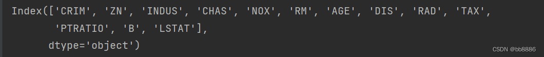
print(data.columns)
print(data.head())

特征（13个）： 

 前几行数据：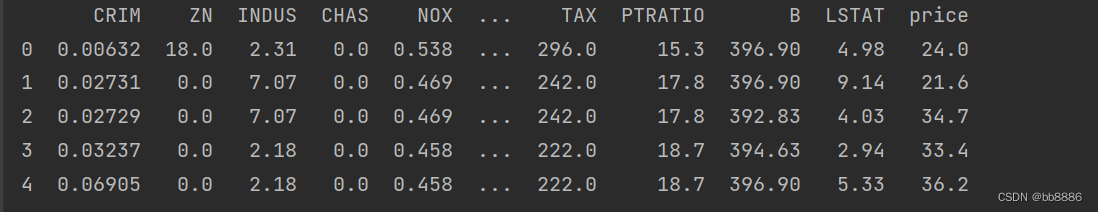

3、拆分特征和标签

y = data.pop('price')

二、数据集处理

1、查看空值

print(data.isnull().sum())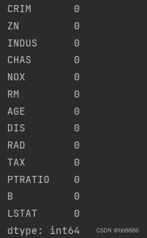

2、查看数据大小

print(data.shape)

3、查看数据描述信息

print(data.describe())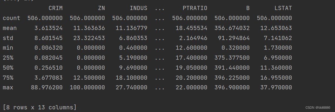

4、划分数据集

x_train, x_test, y_train, y_test = train_test_split(data, y, test_size=0.2, random_state=14)

三、XGBoost建模两种方式以及cv建模

 1、用XGBoost库中的sklearn的API(使用fit和predict)

xgboost参数解释：

不可优化参数：

'booster':'gbtree'--树模型，gblinear--线性模型

'objective': 'multi:softmax'--多分类，'binary:logistic'--二分类，'reg:squarederror'--回归

'nthread':控制线程数目

'silent':设置成1则没有运行信息输出，最好是设置为0.

可优化参数：

'max_depth':树的最大深度。增加这个值会使模型更加复杂，也容易出现过拟合，深度3-10是合理的。

n_estimators: 构建多少颗数 ，树越多越容易过拟合。

'subsample': 每次迭代用多少数据集 0~1。

'colsample_bytree':每次用多少特征 ，可以控制过拟合。

'min_child_weight':树的最小权重 ，越小越容易过拟合。

'learning_rate'/'eta': 学习率, 范围0-1 。默认值 为0.3 , 常用值0.01-0.2。

'gamma':损失下降多少才进行分裂，gammar越大越不容易过拟合。

alpha：控制模型复杂度的权重值的L1正则化项参数，默认为0。

'lambda':控制模型复杂度的权重值的L2正则化项参数，参数越大，模型越不容易过拟合。

# 使用默认参数
params = {'objective': 'reg:squarederror',  # 用来回归任务
          'colsample_bytree': 0.3,  # 每次用多少特征
          'learning_rate': 0.1,
          'max_depth': 5,
          'n_estimators': 10,
          'alpha': 10  # l1正则
          }
xg_reg = xgb.XGBRegressor(**params)
xg_reg.fit(x_train, y_train)
pred = xg_reg.predict(x_test)
print('sklearn API 建模', mean_squared_error(pred, y_test))

2、用XGBoost自身的库来实现（使用train）

用train建模时，参数设置中不需要n_estimators，因为train函数中有一个参数num_boost_round与n_estimators相同的意思。

dtrain = xgb.DMatrix(x_train, label=y_train)
dtest = xgb.DMatrix(x_test, label=y_test)
params = {'objective': 'reg:squarederror',  # 用来回归任务
          'colsample_bytree': 0.3,  # 每次用多少特征
          'learning_rate': 0.1,
          'max_depth': 5,
          'alpha': 10  # l1正则
          }
# num_boost_round:迭代次数，相当于树的个数n_estimators
model = xgb.train(params, dtrain, num_boost_round=10)
pred = model.predict(dtest)
print('xgboost trian 建模：', mean_squared_error(pred, y_test))

不同建模方式的损失值相同： 

3、XGBoost的CV建模

xgboost.cv： 主要提供了一种交叉验证的方式，在每一次迭代中使用交叉验证，并返回理想的决策树数量。

CV参数解释：

dtrain：使用xgb.DMatrix函数得到的训练集

params：对xgboost训练器的参数设置

nfold：交叉验证的折数

early_stopping_round：设置迭代多少次模型没有提升后就结束

num_boost_round：加入的决策树的数目

feaval：自定义的误差函数

data_matrix = xgb.DMatrix(data, y)
params = {"objective": "reg:squarederror",
          "colsample_bytree": 0.3,
          "learning_rate": 0.1,
          "max_depth": 5,
          "alpha": 10}
# xgb.cv--k折交叉验证
cv_results = xgb.cv(dtrain=data_matrix, params=params, nfold=3,
                    num_boost_round=500, early_stopping_rounds=10, metrics="rmse", as_pandas=True, seed=123)
print(cv_results.head())
print((cv_results["test-rmse-mean"]).tail(1))
plt.show()

 

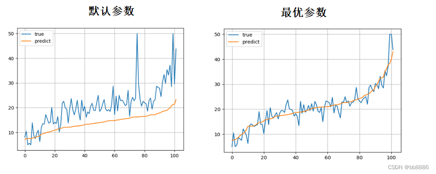
可视化预测值和真实值的折线图

# 预测值与真实值的可视化
y_test = tuple(y_test)
test = []
pre = []
for i in np.argsort(pred):
    test.append(y_test[i])
    pre.append(pred[i])
plt.plot(test, label='true')
plt.plot(pre, label='predict')
plt.legend()
plt.grid()
plt.show()

4、XGBoost的可视化树

# plt方法出来的图太模糊
# import matplotlib.pyplot as plt
# xgb.plot_tree(xg_reg, num_trees=0)
# plt.rcParams['figure.figsize'] = [80, 60]
# plt.show()
# 使用to_graphviz可视化（num_trees：可视化第几棵树，rankdir：从左往右‘LR’还是从上往下’UD‘画树）
graph1 = xgb.to_graphviz(xg_reg, num_trees=9, rankdir='UD')
graph2 = xgb.to_graphviz(model, num_trees=9, rankdir='UD')
graph1.render('./boston')
graph2.render('./boston')

可视化第10棵树： 

5、打印特征权重

如果特征当中有一个权重特别重要，说明有过拟合的风险，或者有穿越的现象。

xgb.plot_importance(xg_reg)
plt.rcParams['figure.figsize'] = [3, 3]
plt.show()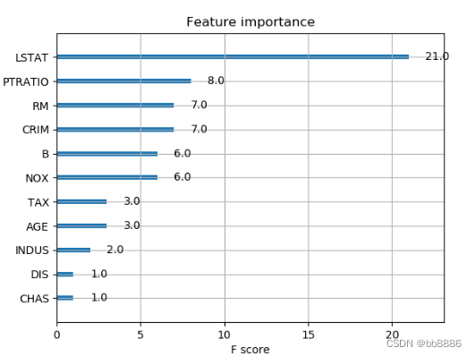

四、XGBoost模型优化

在特征选好、基础模型选好以后我们可以通过调整模型的参数来提高模型准确率。GridSeachCV：组合不同参数的取值，然后输出效果最好的一组参数。

GridSearchCV参数解释：

estimator：所使用的基础模型

param_grid：所需调整的参数，以字典或列表的形式表示

scoring：准确率评判标准

n_jobs：并行运算数量，默认为1

cv：交叉验证折叠数，默认是3，当estimator是分类器时默认使用StratifiedKFold交叉方法，其他问题则默认使用KFold

GridSearchCV属性：

cv_results_:用来输出cv结果的，可以是字典形式也可以是numpy形式，还可以转换成DataFrame格式

best_estimator_：通过搜索参数得到的最好的估计器，当参数refit=False时该对象不可用 best_score_：float类型，输出最好的成绩

best_params_:通过网格搜索得到的score最好对应的参数

GridSearchCV方法：

decision_function(X):返回决策函数值（比如svm中的决策距离）

predict_proba(X):返回每个类别的概率值（有几类就返回几列值）

predict(X)：返回预测结果值（0/1）

score(X, y=None):返回函数

get_params(deep=True):返回估计器的参数

fit(X,y=None,groups=None,fit_params)：在数据集上运行所有的参数组合

transform(X):在X上使用训练好的参数

一般Xgboost调优的顺序可以参考如下：

确定一个较大的学习速率0.1--->num_boost_round（n_estimators）调优--->max_depth 和 min_weight 参数调优-->gamma参数调优-->subsample和colsample_bytree调优-->正则化参数调优-->降低学习速率

1、保持learning rate和其他booster相关的参数不变，调节n_estimator=500。

调节n_estimators可通过xgb.cv得到最优迭代次数即num_boost_round。

cv_params = {'n_estimators': [400, 500, 600, 700, 800]}
params = {'learning_rate': 0.1, 'n_estimators': 500, 'max_depth': 5,
          'min_child_weight': 1, 'seed': 0, 'subsample': 0.8, 'colsample_bytree': 0.8,
          'gamma': 0, 'reg_alpha': 0, 'reg_lambda': 1}

model = xgb.XGBRegressor(**params)
optimized_GBM = GridSearchCV(estimator=model, param_grid=cv_params, scoring='r2', cv=5, verbose=1, n_jobs=4)
optimized_GBM.fit(x_train, y_train)
pred = optimized_GBM.predict(x_test)
# 输出最佳参数
print(optimized_GBM.best_params_)
print(mean_squared_error(pred, y_test))
print(optimized_GBM.best_score_)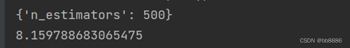

2、调节booster相关参数（max_depth and min_child_weight、gamma、subsample以及colsample_bytree、reg_alpha以及reg_lambda）

2.1 调节max_depth=4, min_child_weight=3。

cv_params = {'max_depth': [3, 4, 5, 6, 7],
             'min_child_weight': [1, 2, 3]
             }
params = {'learning_rate': 0.1, 'n_estimators': 500, 'max_depth': 5,
          'min_child_weight': 1, 'seed': 0, 'subsample': 0.8, 'colsample_bytree': 0.8,
          'gamma': 0, 'reg_alpha': 0, 'reg_lambda': 1}

2.2 调节gamma=0.4 gamma用来控制树的生长。

cv_params = {'gamma': [0.1, 0.2, 0.3, 0.4, 0.5, 0.6]}
params = {'learning_rate': 0.1, 'n_estimators': 500, 'max_depth': 4,
          'min_child_weight': 3, 'seed': 0, 'subsample': 0.8, 'colsample_bytree': 0.8,
          'gamma': 0, 'reg_alpha': 0, 'reg_lambda': 1}

 

2.3 调节subsample=0.8以及colsample_bytree=0.9。

cv_params = {'subsample': [0.5, 0.6, 0.7, 0.8, 0.9, 1],  # 每次迭代用多少数据集
             'colsample_bytree': [0.5, 0.6, 0.7, 0.8, 0.9, 1]
             }
params = {'learning_rate': 0.1, 'n_estimators': 500, 'max_depth': 4,
          'min_child_weight': 3, 'seed': 0, 'subsample': 0.8, 'colsample_bytree': 0.8,
          'gamma': 0.4, 'reg_alpha': 0, 'reg_lambda': 1}

2.4 调节reg_alpha=0.25 以及reg_lambda=1。

cv_params = {'reg_alpha': [0, 0.25, 0.5, 0.75, 1],
             'reg_lambda': [0, 0.25, 0.5, 0.75, 1]
             }
params = {'learning_rate': 0.1, 'n_estimators': 500, 'max_depth': 4,
          'min_child_weight': 3, 'seed': 0, 'subsample': 0.8, 'colsample_bytree': 0.9,
          'gamma': 0.4, 'reg_alpha': 0, 'reg_lambda': 1}

3、调节learning_rate=0.05

cv_params = {'learning_rate': [0.01, 0.05, 0.07]}
params = {'learning_rate': 0.1, 'n_estimators': 500, 'max_depth': 4,
          'min_child_weight': 3, 'seed': 0, 'subsample': 0.8, 'colsample_bytree': 0.9,
          'gamma': 0.4, 'reg_alpha': 0.25, 'reg_lambda': 1}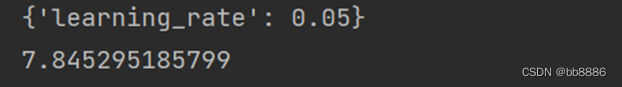

4、最后用调整后的参数创建模型

params = {'learning_rate': 0.05, 'n_estimators': 500, 'max_depth': 4,
        'min_child_weight': 3, 'seed': 0, 'subsample': 0.8, 'colsample_bytree': 0.9,
        'gamma': 0.4, 'reg_alpha': 0.25, 'reg_lambda': 1}
xg_reg = xgb.XGBRegressor(**params)
xg_reg.fit(x_train, y_train)
pred = xg_reg.predict(x_test)
print(mean_squared_error(pred, y_test))