TensorFlow 实现Boston房价预测

综述

本文使用了 TensorFlow 2.0 框架，搭建了 ANN（人工神经网络），实现 Boston 房价预测。本文使用的编程工具为 jupyter notebook，完整代码可以在我的GitHub中找到，GitHub链接在此

Boston 房价预测，是一个非常经典的案例了，已有许多学者对其进行了各式各样的研究，也通过拟合各种各样的模型，对该问题做出了实现。

通过该案例，我相信你一定能进一步的学习到 TensorFlow 2.0 下的 ANN 的搭建，相信你可以通过该案例，有所收益。

代码与解释

导入所需的库函数

import tensorflow as tf
import numpy as np
import pandas as pd
import matplotlib as mpl
import matplotlib.pyplot as plt
%matplotlib inline
import sklearn

读入数据，并查看数据维度

from sklearn.datasets import fetch_california_housing

housing = fetch_california_housing()
print(housing.data.shape)
print(housing.target.shape)

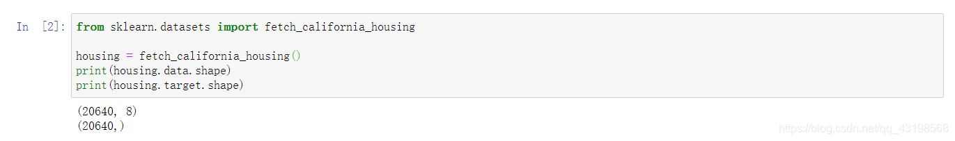
由图可得，数据一共有20640条，其中自变量数据有20640行、8列的数据。

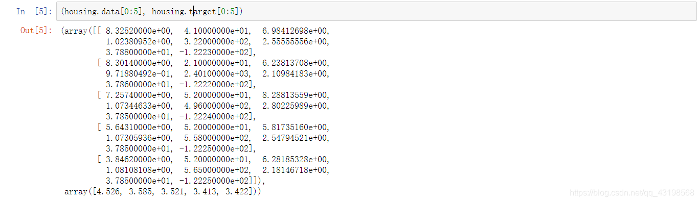
部分数据查看，查看前五条数据

print((housing.data[0:5], housing.target[0:5]))

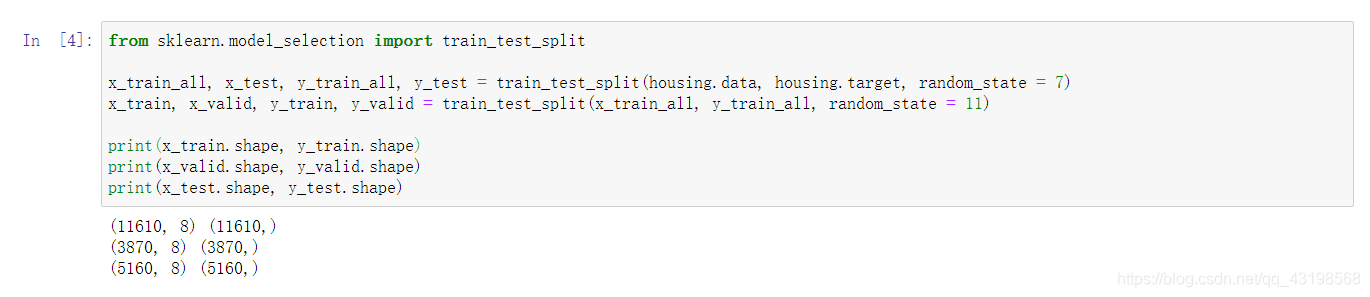
数据拆分，1/4分

from sklearn.model_selection import train_test_split

x_train_all, x_test, y_train_all, y_test = train_test_split(housing.data, housing.target, random_state = 7)
x_train, x_valid, y_train, y_valid = train_test_split(x_train_all, y_train_all, random_state = 11)

print(x_train.shape, y_train.shape)
print(x_valid.shape, y_valid.shape)
print(x_test.shape, y_test.shape)

数据归一化处理

from sklearn.preprocessing import StandardScaler

scaler = StandardScaler()
x_train_scaled = scaler.fit_transform(x_train)
x_vaild_scaled = scaler.transform(x_valid)
x_test_scaled = scaler.transform(x_test)

神经网络搭建

model = tf.keras.Sequential(
    [tf.keras.layers.Dense(60, activation = 'relu', input_shape = x_train.shape[1:]),
     tf.keras.layers.Dense(120, activation = 'relu'),
     tf.keras.layers.Dense(240, activation = 'relu'),
     tf.keras.layers.Dense(480, activation = 'relu'),
     tf.keras.layers.Dense(240, activation = 'relu'),
     tf.keras.layers.Dense(120, activation = 'relu'),
     tf.keras.layers.Dense(60, activation = 'relu'),
     tf.keras.layers.Dense(1)]
)

model.summary()

设置优化模型、损失函数、回调函数

model.compile(optimizer = 'adam', loss = 'mse')
callbacks = [keras.callbacks.EarlyStopping(patience = 5, min_delta = 1e-3)]

模型训练

history = model.fit(x_train_scaled, y_train, validation_data = (x_vaild_scaled, y_valid), epochs = 3000, callbacks = callbacks)

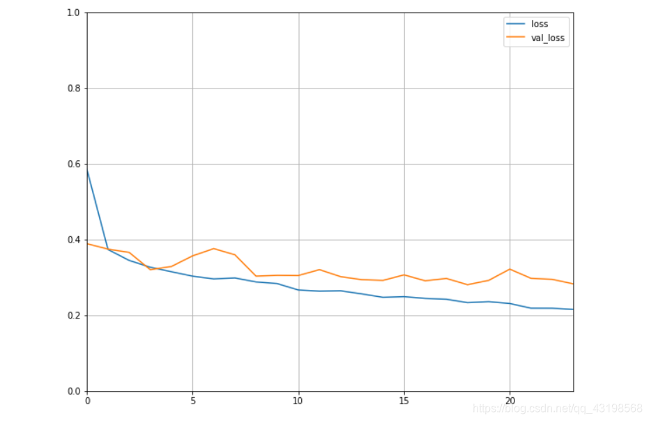
可视化损失值

def plot_learning_curver(history):
    pd.DataFrame(history.history).plot(figsize = (10, 8))
    plt.grid(True)
    plt.gca().set_ylim(0, 1)

plot_learning_curver(history)

测试集，模型结果测试

model.evaluate(x_test_scaled, y_test, verbose=0)

关键点

关键点1：
输入层即第一层，输入的维度，一定要正确，要和你的数据维度相匹配，不然模型训练时，就会无法进行。
关键点2：
输出层即最后一层，有多少种结果，就有多少结点，此处的结点数一定不能随意设置。
关键点3：
除开上述两点，中间层的结点数可以随意设置，中间层数也可以随意设置，但是需要注意，设置的层数越多、结点数越多，计算量就越大，就越耗费时间。
关键点4：
对于第三点，还有补充，虽然大多数时间，神经网络越大越深，模型的拟合效果就越好，但是，也会出现一种很严重的问题，那就是过拟合问题，如何解决过拟合问题，有许多方法，在本文中使用的回调函数，就是防止过拟合的手段之一，在TensorFlow中还有着许多的防止过拟合的手段，我会在之后的博客中慢慢讲到。

结语

通过本案例，我相信你对 TensorFlow 搭建神经网络，有了更深的理解，望你在深度学习之旅中，愉快！