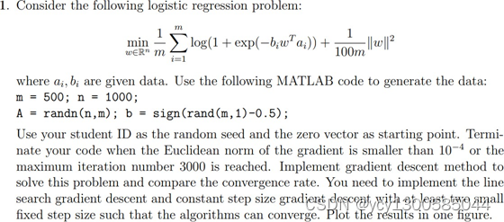
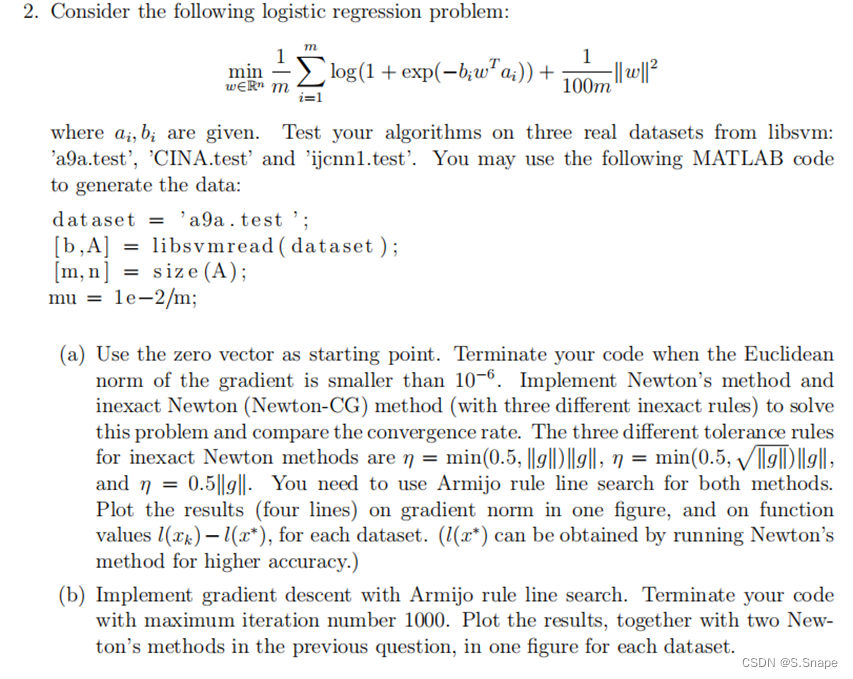
Consider the following Logistic Regression Problem：

$min_{w\in R_{n}}\frac{1}{m}\sum_{i=1}^{m}log(1+exp(-b_{i}w^{T}a_{i}))+\frac{1}{100m}\left \| w \right \|^{2}$

where $a_{i}\in R^{n},b_{i}\in {\{-1,+1\}}$ are given data

这里 $b=(b_{1},b_{2},...,b_{m})^{T}$ 的意义是标签向量

Matlab Code.zip

内附a9a.test、CINA.test和ijcnn1.test数据集，以及libsvmread.mexw64文件，用于读取数据集

如果你不想从CSDN下载(because it sucks)，也可以通过百度网盘下载：

Matlab code.zip (3.16MB)

一、数学形式及其Matlab实现

1. Logistic Regression 损失函数及其梯度的数学表示：

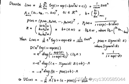
损失函数及其梯度的 Matlab 实现：

function z = Sigmoid(z)
%Sigmoid函数 
    z = 1./(1 + exp(-z)); 
end 
function object = L(w,m0,A,b)
%逻辑回归(Logistic Regression)问题的目标函数(即损失函数)
    object = m0*(sum(log(1+exp(-b.*(A'*w))))+(1/100)*(w'*w)); 
end 
function grad = Gradient(w,m0,A,b)
%目标函数的梯度 
    grad = m0*(-A*(b.*(1-Sigmoid(b.*(A'*w))))+(1/50)*w); 
end

2. 损失函数的 Hessian 矩阵的数学表示：

损失函数的 Hessian 矩阵的 Matlab 实现：

function hess = Hessian(w,m0,n,A,b)
%目标函数的海塞矩阵 
    sigmoid = Sigmoid(b.*(A*w)); 
    vector = sigmoid.*(1-sigmoid); 
%实际上应是 b.*sigmoid.*(1-sigmoid).*b,其中b代表的是逻辑回归问题的标签向量
%由于 b 的元素只能是±1,故左右点乘 b 是不发生任何影响,故可写作 sigmoid.*(1-sigmoid) 
    repeat_vector = repmat(vector',n,1); 
%在行维度和列维度上分别重复 vector 的转置 n 次和 1 次,构造 nxm 的矩阵 repeat_vector 
%用 repeat_vector.*A'*A 代替 A'*diag(vector)*A,如果 m>n 的话可以节省空间 
%而且将一次矩阵乘法变为矩阵点乘，时间复杂度也降低 
    hess = m0*(repeat_vector.*A'*A + diag((1/50)*ones(n,1))); 
end

3. 回溯法的数学形式：

(注： $t_{k}$ 代表步长， $p_{k}$ 代表的是下降方向，k是外层算法的迭代次数，s相当于回溯法的迭代次数)

对于梯度法： $p_{k}=-\triangledown L(x_{k})$

对于牛顿法： $p_{k}=-{\triangledown ^{2}L(x_{k})}^{-1}\triangledown L(x_{k})$

α、β和 $\hat{t}$ 是回溯法的参数，α为一个很小的正数，β∈(0,1)， $\hat{t}$ 是刚开始的步长

回溯法从一个较大的步长 $\hat{t}$ 开始，每次迭代乘以β，即第s次迭代中 $t_{k}=\hat{t}\beta ^{s}$ ，直到找到最小的非负整数s，使得： $L(x_{k}+t_{k}p_{k})\leq L(x_{k})+\alpha t_{k}{p_{k}}^{T}\triangledown L(x_{k})$

对比于精确法确定步长： $t_{k}=argmin_{t\geq 0}L(x_{k}+t{p}_{k})$ ，回溯法确定步长更易实现

回溯法确定步长的 Matlab 实现：

function StepSize = Backtracking(w,m0,A,b,object,grad,direction) 
%回溯法求步长，即找到一个步长使得“新的目标函数值≤原目标函数值+α*步长*<下降方向,梯度>"
%α为一个小的正数(这里取α=1e-4),direction是下降方向,< , >代表向量内积
%找法是从一个较大的步长开始(这里从1开始),每次迭代乘以β,β∈(0,1)(这里取β=0.5),相当于不断往前摸索
%所谓“回溯”可能就是来源于此,相较于精确法确定步长(即解出最优步长),回溯法确定步长更容易实现
%精确线搜索(Exact line search)中使用的步长是下降方向上最优的步长
    alpha = 1e-4;
    beta = 0.5; 
    StepSize = 1; 
    new_w = w + StepSize*direction; 
    while L(new_w,m0,A,b) > (object + alpha * StepSize * (direction' * grad)) 
        StepSize = StepSize * beta; 
        new_w = w + StepSize*direction; 
    end 
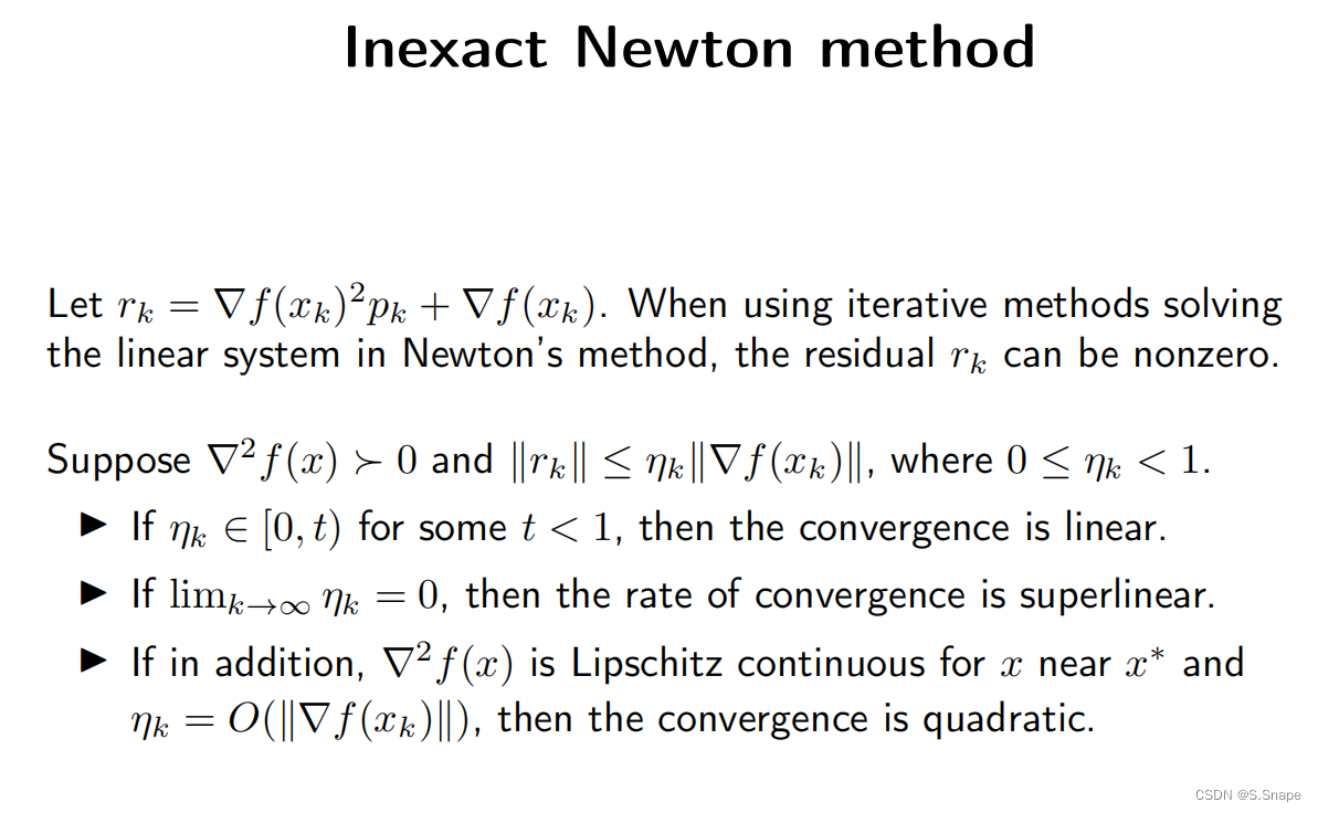
end

4. 精确牛顿法(Exact Newton)与非精确牛顿法(Inexact Newton)的区别

牛顿法的下降方向为 $p_{k}=-{\triangledown ^{2}L(x_{k})}^{-1}\triangledown L(x_{k})$ ，根据其计算方法可分为精确法和非精确法；

精确法是通过计算Hessian矩阵的逆 ${\triangledown ^{2}L(x_{k})}^{-1}$ ，再与梯度 $\triangledown L(x_{k})$ 相乘，最后取负得到 $p_{k}$ ；
而非精确法利用共轭梯度法(Conjugate Gradient,CG)计算下降方向，来规避矩阵求逆的运算量

通过共轭梯度法可以获得线性系统 $Ax=b$ 的近似解 (区别于解析解 $x=A^{-1}b$ )

令 $A={\triangledown ^{2}L(x_{k})}$ ， $x=p_{k}$ ， $b=-\triangledown L(x_{k})$ ，即可获得线性系统 ${\triangledown ^{2}L(x_{k})}p_{k}=-\triangledown L(x_{k})$ 的解

记残差(residual) $r_{k}={\triangledown ^{2}L(x_{k})}p_{k}+\triangledown L(x_{k})$

对于凸问题，共轭梯度法迭代的终止条件为： $\left \| r_{k} \right \|\leqslant\eta _{k}\left \| \bigtriangledown L(x_{k})\right \|$

而 $\eta _{k}$ 有不同的取法，称为非精确规则(Inexact Rule)，常用的三个非精确规则为：

$\eta _{k}=min\{0.5,\left \| \bigtriangledown L(x_{k})\right \|\}$
$\eta _{k}=min\{0.5,\sqrt{\left \| \bigtriangledown L(x_{k})\right \|}\}$
$\eta _{k}=0.5$

显然，从左至右，三个非精确规则对应的非精确牛顿法的收敛速度依次递减

精确牛顿法计算下降方向的代码：

direction = - hess\grad;

非精确法使用的共轭梯度法的代码：

①非精确规则：

function CG_tol = InexactRule(ng)
%共轭梯度法的inexact rule
    CG_tol = zeros(3,1);
    CG_tol(1) = min(0.5,ng)*ng;
    CG_tol(2) = min(0.5,sqrt(ng))*ng;
    CG_tol(3) = 0.5*ng;
end

②CG：

function x = CG(A,g,ng,CG_MaxIter,Rule)
%共轭梯度法，解方程Ax=-g，ng为g的二范数,Rule为使用的inexact rule的编号
%对于牛顿法，A=Hessian，g=gradient，ng=norm(gradient,2),x为近似牛顿方向
    x = 0;
    CG_tol = InexactRule(ng);
%残差(residual)=Ax+g,不妨设下降方向的初值是零向量,则残差的初值是g
    r = g;
    p = -r;
    for iter = 1:CG_MaxIter
        rr = r' * r;
        Ap = A * p;
        alpha = rr / (p'*Ap);
        x = x + alpha * p;
        r = r + alpha * Ap;
        nrl = norm(r);
        if nrl <= CG_tol(Rule)
           break;
        end
        beta = nrl^2 / rr;
        p = -r + beta * p;
    end
    fprintf('Number of CG iteration:\t%d\n',iter); %设置输出语句方便调试
end

二、第1题：

结果：

代码：

id = mod(21307140051,pow2(32));
%对于rng()来说学号太大，故可取模2^32的余数，来设置种子
rng(id,'twister');
%随机数模式为twister，用rand('seed',id)设置种子似乎并不能使随机数结果复现

m = 500;
m0 = 1/m;%优化，用于减少1/m运算的次数
n = 1000;
w = zeros(n,1);%自变量
A = randn(n,m);%参量
b = sign(rand(m,1)-0.5);
i = zeros(3,1);%i用于记录三次梯度法的迭代次数

fprintf("Constant Stepsize(0.02) Gradient Method:\n");
[history1,i(1)] = ConstantStepSizeGradient(w,m0,A,b,0.02,3000,1e-4);
%执行固定步长为0.02的梯度法，最多迭代3000次
fprintf("result = %f\twith %d steps\n",history1(i(1)+1,1),i(1));

fprintf("Constant Stepsize(0.04) Gradient Method:\n");
[history2,i(2)] = ConstantStepSizeGradient(w,m0,A,b,0.04,3000,1e-4);
%执行固定步长为0.04的梯度法，最多迭代3000次
fprintf("result = %f\twith %d steps\n",history2(i(2)+1,1),i(2));

fprintf("Backtracking Gradient Method:\n");
[history3,i(3)] = BacktrackingGradient(w,m0,A,b,3000,1e-4);
%执行回溯线搜索，最多迭代3000次,终止条件为梯度的二范数小于1e-4
fprintf("result = %f\twith %d steps\n",history3(i(3)+1,1),i(3));

%打印三个算法终止时的目标函数值以及迭代次数
fprintf(['Constant step size 0.02:\t%f\t(%d iteration)\n' ...
         'Constant step size 0.04:\t%f\t(%d iteration)\n' ...
         'Backtracking line search(t_hat = 1,alpha = 0.001,beta = 0.5):\t' ...
         '%f\t(%d iteration)\n'], ...
         history1(i(1)+1,1),i(1), ...
         history2(i(2)+1,1),i(2), ...
         history3(i(3)+1,1),i(3));

%创建绘图窗口
figure
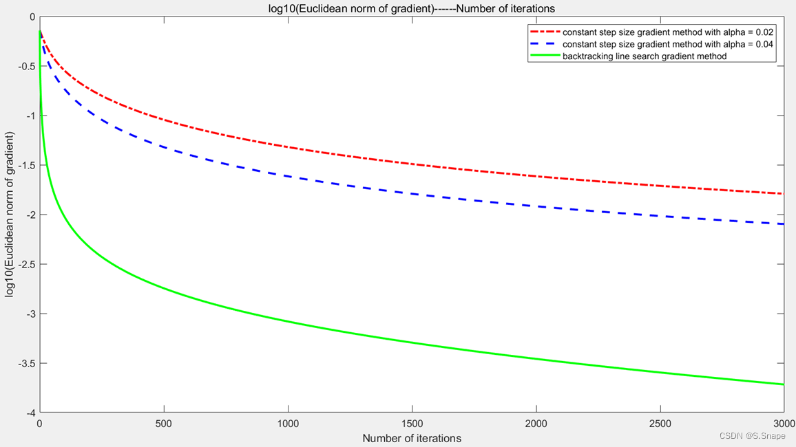
%绘制“log10(梯度范数)---迭代次数”的图像
plot(0:i(1),log10(history1(1:i(1)+1,2)),'-.r', ...%设置了线型和颜色分别为
     0:i(2),log10(history2(1:i(2)+1,2)),'--b', ...%"实线绿色"、"虚线蓝色"和"点线红色"
     0:i(3),log10(history3(1:i(3)+1,2)),'-g','LineWidth',2)%设置了线宽为2磅(默认值的4倍)
%添加图例
legend('constant step size gradient method with alpha = 0.02', ...
       'constant step size gradient method with alpha = 0.04', ...
       'backtracking line search gradient method')
%添加标题
title('log10(Euclidean norm of gradient)------Number of iterations')
%添加坐标轴标签
xlabel('Number of iterations')
ylabel('log10(Euclidean norm of gradient)')

function z = Sigmoid(z)
%Sigmoid函数
    z = 1./(1 + exp(-z));
end

function object = L(w,m0,A,b)
%逻辑回归(Logistic Regression)问题的目标函数
    object = m0*(sum(log(1+exp(-b.*(A'*w))))+(1/100)*(w'*w));
end

function grad = Gradient(w,m0,A,b)
%目标函数的梯度
    grad = m0*(-A*(b.*(1-Sigmoid(b.*(A'*w))))+(1/50)*w);
end

function [history,i] = ConstantStepSizeGradient(w,m0,A,b,StepSize,Iteration,epsilon)
%固定步长为StepSize的梯度法，最多迭代Iteration次，终止条件为梯度的二范数小于epsilon    
    history = zeros(Iteration+1,2);
    for i = 1:Iteration
        object = L(w,m0,A,b);
        history(i,1) = object;
        grad = Gradient(w,m0,A,b);
        w = w - StepSize*grad; %update w, 固定步长
        history(i,2) = norm(grad);
        if history(i,2) < epsilon %Termination Criteria
           break
        end
        if mod(i,500)==0 %设置输出语句方便调试
           fprintf('Number of Iteration:\t%d\n',i);
        end
    end
    history(i+1,1) = L(w,m0,A,b); %若总共迭代i次，则会将i+1个目标函数值写入history的第一列
    grad = Gradient(w,m0,A,b);
    history(i+1,2) = norm(grad); %将i+1个梯度范数值写入history的第二列
end

function StepSize = Backtracking(w,m0,A,b,object,grad,direction)
%回溯法求步长，即找到一个步长使得“新的目标函数值≤原目标函数值+α*步长*<下降方向,梯度>"
%α为一个小的正数(这里取α=1e-4),direction是下降方向,< , >代表向量内积
%找法是从一个较大的步长开始(这里从1开始),每次迭代乘以β,β∈(0,1)(这里取β=0.5),相当于不断往前摸索
%所谓“回溯”可能就是来源于此,相较于精确法确定步长(即解出最优步长),回溯法确定步长更容易实现
%精确线搜索(Exact line search)中使用的步长是下降方向上最优的步长
    alpha = 1e-4;
    beta = 0.5;
    StepSize = 1;
    new_w = w + StepSize*direction;
    while L(new_w,m0,A,b) > (object + alpha * StepSize * (direction' * grad))
        StepSize = StepSize * beta;
        new_w = w + StepSize*direction;
    end
end

function [history,i] = BacktrackingGradient(w,m0,A,b,Iteration,epsilon)
%回溯线搜索，最多迭代Iteration次，终止条件为梯度的二范数小于epsilon
    history = zeros(Iteration+1,2);
    for i = 1:Iteration
        object = L(w,m0,A,b);
        history(i,1) = object;
        grad = Gradient(w,m0,A,b);
        direction = -grad; %下降方向
        StepSize = Backtracking(w,m0,A,b,object,grad,direction); %回溯法确定步长
        w = w + StepSize*direction; %update w
        history(i,2) = norm(grad);
        if history(i,2) < epsilon %终止条件(Termination Criteria)
           break
        end
        if mod(i,500)==0 %设置输出语句方便调试
           fprintf('Number of Iteration:\t%d\n',i);
        end
    end
    history(i+1,1) = L(w,m0,A,b); %若总共迭代i次，则会将i+1个目标函数值写入history的第一列
    grad = Gradient(w,m0,A,b);
    history(i+1,2) = norm(grad); %将i+1个梯度范数值写入history的第二列
end

三、第2题：

加载a9a.test数据集的Matlab语句：

dataset = 'a9a.test';
[b,A] = libsvmread(dataset);

加载CINA.test和ijcnn1.test数据集只需要对第一个语句做相应的修改即可；

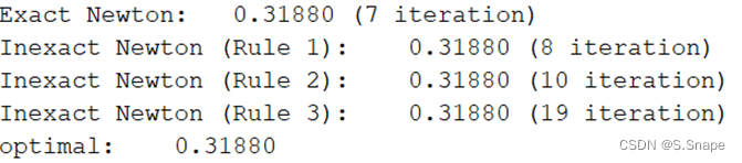
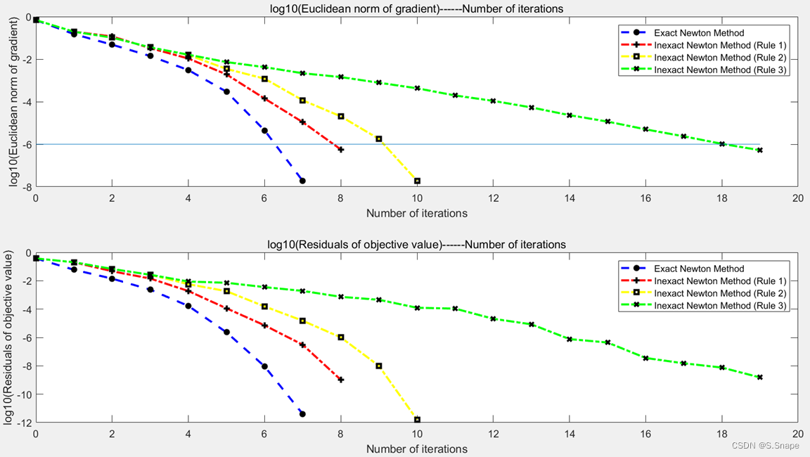
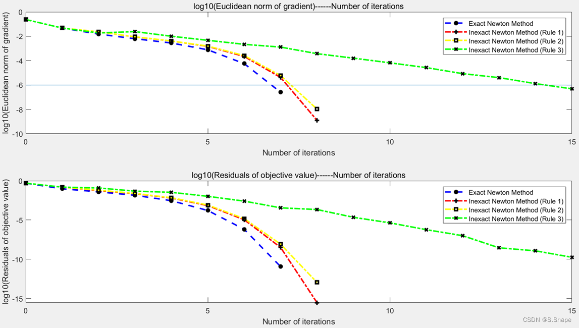
1. 第二题(a):

结果：

①a9a.test:

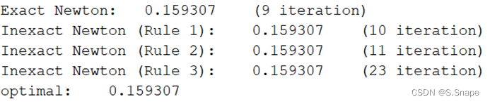
②CINA.test:

③ijcnn1.test:

代码：

%读取数据集
dataset = 'a9a.test';
[b,A] = libsvmread(dataset);

[m,n] = size(A);
m0 = 1/m;
w = zeros(n,1);
i = zeros(6,1);

%为保持与第二题(b)的对齐,编号为1的history和i保留
fprintf('Exact Newton:\n');
[history2,i(2)] = ExactNewton(w,m0,n,A,b,1e-6);
%精度为1e-6的精确牛顿法
fprintf('result = %f\twith %d steps\n',history2(i(2)+1,1),i(2));

fprintf('Inexact Newton (Rule 1):\n');
[history3,i(3)] = InexactNewton(w,m0,n,A,b,1e-6,1000,1);
%精度为1e-6、CG最大迭代次数为1000、使用第1条规则的非精确牛顿法
fprintf('result = %f\twith %d steps\n',history3(i(3)+1,1),i(3));

fprintf('Inexact Newton (Rule 2):\n');
[history4,i(4)] = InexactNewton(w,m0,n,A,b,1e-6,1000,2);
%精度为1e-6、CG最大迭代次数为1000、使用第2条规则的非精确牛顿法
fprintf('result = %f\twith %d steps\n',history4(i(4)+1,1),i(4));

fprintf('Inexact Newton (Rule 3):\n');
[history5,i(5)] = InexactNewton(w,m0,n,A,b,1e-6,1000,3);
%精度为1e-6、CG最大迭代次数为1000、使用第3条规则的非精确牛顿法
fprintf('result = %f\twith %d steps\n',history5(i(5)+1,1),i(5));

fprintf('Exact Newton with higher accuracy:\n');
[history6,i(6)] = ExactNewton(w,m0,n,A,b,1e-12);
%精度为1e-12的精确牛顿法,以此近似最优值
fprintf('result = %f\twith %d steps\n',history6(i(6)+1,1),i(6));

%以更高精度的牛顿法的结果作为最优值的近似值
optimal = history6(i(6)+1,1);
%打印算法终止时的目标函数值以及迭代次数
fprintf(['Exact Newton:\t%6.5f\t(%d iteration)\n' ...
         'Inexact Newton (Rule 1):\t%6.5f\t(%d iteration)\n' ...
         'Inexact Newton (Rule 2):\t%6.5f\t(%d iteration)\n' ...
         'Inexact Newton (Rule 3):\t%6.5f\t(%d iteration)\n' ...
         'optimal:\t%6.5f\n'], ...
         history2(i(2)+1,1),i(2), ...
         history3(i(3)+1,1),i(3), ...
         history4(i(4)+1,1),i(4), ...
         history5(i(5)+1,1),i(5), ...
         optimal);

%创建绘图窗口
figure

%子图1,绘制“log10(梯度范数)-迭代数”图
subplot(2,1,1);
plot(0:i(2),log10(history2(1:i(2)+1,2)),'b--*', ...
     0:i(3),log10(history3(1:i(3)+1,2)),'r-.+', ...
     0:i(4),log10(history4(1:i(4)+1,2)),'y-.s', ...
     0:i(5),log10(history5(1:i(5)+1,2)),'g-.x', ...
     'LineWidth',2 ,'MarkerEdgeColor','k','MarkerSize',6);
%添加直线y=-6
line(0:i(5),-6*ones(i(5)+1,1));
%添加图例
legend('Exact Newton Method', ...
       'Inexact Newton Method (Rule 1)', ...
       'Inexact Newton Method (Rule 2)', ...
       'Inexact Newton Method (Rule 3)');
%添加标题
title('log10(Euclidean norm of gradient)------Number of iterations')
%添加坐标轴标签
xlabel('Number of iterations')
ylabel('log10(Euclidean norm of gradient)')

%子图2,绘制log10(残差)-迭代数图
subplot(2,1,2);
plot(0:i(2),log10(history2(1:i(2)+1,1)-optimal),'b--*', ...
     0:i(3),log10(history3(1:i(3)+1,1)-optimal),'r-.+',...
     0:i(4),log10(history4(1:i(4)+1,1)-optimal),'y-.s',...
     0:i(5),log10(history5(1:i(5)+1,1)-optimal),'g-.x',...
     'LineWidth',2 ,'MarkerEdgeColor','k','MarkerSize',6);
%添加图例
legend('Exact Newton Method', ...
       'Inexact Newton Method (Rule 1)', ...
       'Inexact Newton Method (Rule 2)', ...
       'Inexact Newton Method (Rule 3)');
%添加标题
title('log10(Residuals of objective value)------Number of iterations')
%添加坐标轴标签
xlabel('Number of iterations')%添加坐标轴标签
ylabel('log10(Residuals of objective value)')

function z = Sigmoid(z)
%Sigmoid函数
    z = 1./(1 + exp(-z));
end

function object = L(w,m0,A,b)
%逻辑回归(Logistic Regression)问题的目标函数
    object = m0*(sum(log(1+exp(-b.*(A*w))))+(1/100)*(w'*w));
end

function grad = Gradient(w,m0,A,b)
%目标函数的梯度
    grad = m0*(-A'*(b.*(1-Sigmoid(b.*(A*w))))+(1/50)*w);
end

function hess = Hessian(w,m0,n,A,b)
%目标函数的海塞矩阵
    sigmoid = Sigmoid(b.*(A*w));
    vector = sigmoid.*(1-sigmoid);
%实际上应是b.*sigmoid.*(1-sigmoid).*b
%但由于b的元素只能是±1,故左右点乘b是不发生任何影响,故可写作sigmoid.*(1-sigmoid)
    repeat_vector = repmat(vector',n,1);
%在行维度和列维度上分别重复vector的转置n次和1次,构造nxm的矩阵repeat_vector
%用repeat_vector.*A'*A代替A'*diag(vector)*A,如果m>n的话可以节省空间
%而且将一次矩阵乘法变为矩阵点乘，时间复杂度也降低
    hess = m0*(repeat_vector.*A'*A + diag((1/50)*ones(n,1)));
end

function StepSize = Backtracking(w,m0,A,b,object,grad,direction)
%回溯法求步长，即找到一个步长使得“新的目标函数值≤原目标函数值+α*步长*<下降方向,梯度>"
%α为一个小的正数(这里取α=1e-4),direction是下降方向,< , >代表向量内积
%找法是从一个较大的步长开始(这里从1开始),每次迭代乘以β,β∈(0,1)(这里取β=0.5),相当于不断往前摸索
%所谓“回溯”可能就是来源于此,相较于精确法确定步长(即解出最优步长),回溯法确定步长更容易实现
%精确线搜索(Exact line search)中使用的步长是下降方向上最优的步长
    alpha = 1e-4;
    beta = 0.5;
    StepSize = 1;
    new_w = w + StepSize*direction;
    while L(new_w,m0,A,b) > (object + alpha * StepSize * (direction' * grad))
        StepSize = StepSize * beta;
        new_w = w + StepSize*direction;
    end
end

function [history,i] = ExactNewton(w,m0,n,A,b,epsilon)
%精确牛顿法，精度要求为epsilon
    history = zeros(1001,2);
    i = 0;
    object = L(w,m0,A,b);
    history(i+1,1) = object;
    grad = Gradient(w,m0,A,b);
    hess = Hessian(w,m0,n,A,b);
    direction = -hess\grad; %精确下降方向
    StepSize = Backtracking(w,m0,A,b,object,grad,direction); %回溯法确定步长
    w = w + StepSize*direction;
    history(i+1,2) = norm(grad);
    fprintf('%d iteration done!\n',i+1);
    while history(i+1,2) >= epsilon
          i = i + 1;
          object = L(w,m0,A,b);
          history(i+1,1) = object;
          grad = Gradient(w,m0,A,b);
          hess = Hessian(w,m0,n,A,b);
          direction = -hess\grad; %精确下降方向
          StepSize = Backtracking(w,m0,A,b,object,grad,direction); %回溯法确定步长
          w = w + StepSize*direction;
          history(i+1,2) = norm(grad);
          fprintf('%d iteration done!\n',i+1); %设置输出语句方便调试
    end
end

function CG_tol = InexactRule(ng)
%共轭梯度法的inexact rule
    CG_tol = zeros(3,1);
    CG_tol(1) = min(0.5,ng)*ng;
    CG_tol(2) = min(0.5,sqrt(ng))*ng;
    CG_tol(3) = 0.5*ng;
end

function x = CG(A,g,ng,CG_MaxIter,Rule)
%共轭梯度法，解方程Ax=-g，ng为g的二范数,Rule为使用的inexact rule的编号
%对于牛顿法，A=Hessian，g=gradient，ng=norm(gradient,2),x为近似牛顿方向
    x = 0;
    CG_tol = InexactRule(ng);
    r = g;
    p = -r;
    for iter = 1:CG_MaxIter
        rr = r' * r;
        Ap = A * p;
        alpha = rr / (p'*Ap);
        x = x + alpha * p;
        r = r + alpha * Ap;
        nrl = norm(r);
        if nrl <= CG_tol(Rule)
           break;
        end
        beta = nrl^2 / rr;
        p = -r + beta * p;
    end
    fprintf('Number of CG iteration:\t%d\n',iter); %设置输出语句方便调试
end

function [history,i] = InexactNewton(w,m0,n,A,b,epsilon,CG_MaxIter,Rule)
%非精确牛顿法，精度要求为epsilon，每次迭代中CG的最大迭代次数为CG_MaxIter
%Rule为使用的inexact rule的编号
    history = zeros(1001,2);
    i = 0;
    object = L(w,m0,A,b);
    history(i+1,1) = object;
    grad = Gradient(w,m0,A,b);
    hess = Hessian(w,m0,n,A,b);
    norm_grad = norm(grad);
    direction = CG(hess,grad,norm_grad,CG_MaxIter,Rule); %CG法计算近似下降方向
    StepSize = Backtracking(w,m0,A,b,object,grad,direction); %回溯法确定步长
    w = w + StepSize*direction;
    history(i+1,2) = norm_grad;
    while history(i+1,2) >= epsilon
          i = i + 1;
          object = L(w,m0,A,b);
          history(i+1,1) = object;
          grad = Gradient(w,m0,A,b);
          hess = Hessian(w,m0,n,A,b);
          norm_grad = norm(grad);
          direction = CG(hess,grad,norm_grad,CG_MaxIter,Rule); %CG法计算近似下降方向
          StepSize = Backtracking(w,m0,A,b,object,grad,direction); %回溯法确定步长
          w = w + StepSize*direction;
          history(i+1,2) = norm_grad;
    end
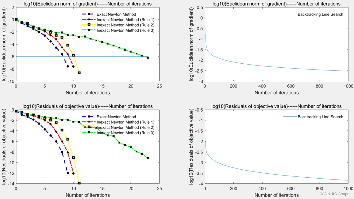
end

2. 第2题(b):

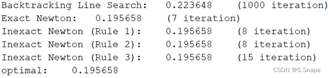
结果：

①a9a.test：

②CINA.test：

③ijcnn1.test

代码：

(与(a)中代码的区别主要是前面输入和绘图的指令，并添加了BacktrackingGradient函数)

%读取数据集
dataset = 'a9a.test';
[b,A] = libsvmread(dataset);

[m,n] = size(A);
m0 = 1/m;
w = zeros(n,1);
i = zeros(6,1);

fprintf('Backtracking Gradient:\n');
[history1,i(1)] = BacktrackingGradient(w,m0,A,b,1000);
%未设置精度要求的回溯线搜索，迭代1000次
fprintf('result = %f\twith %d steps\n',history1(i(1)+1,1),i(1));

fprintf('Exact Newton:\n');
[history2,i(2)] = ExactNewton(w,m0,n,A,b,1e-6);
%精度为1e-6的精确牛顿法
fprintf('result = %f\twith %d steps\n',history2(i(2)+1,1),i(2));

fprintf('Inexact Newton (Rule 1):\n');
[history3,i(3)] = InexactNewton(w,m0,n,A,b,1e-6,1000,1);
%精度为1e-6、CG最大迭代次数为1000、使用第1条规则的非精确牛顿法
fprintf('result = %f\twith %d steps\n',history3(i(3)+1,1),i(3));

fprintf('Inexact Newton (Rule 2):\n');
[history4,i(4)] = InexactNewton(w,m0,n,A,b,1e-6,1000,2);
%精度为1e-6、CG最大迭代次数为1000、使用第2条规则的非精确牛顿法
fprintf('result = %f\twith %d steps\n',history4(i(4)+1,1),i(4));

fprintf('Inexact Newton (Rule 3):\n');
[history5,i(5)] = InexactNewton(w,m0,n,A,b,1e-6,1000,3);
%精度为1e-6、CG最大迭代次数为1000、使用第3条规则的非精确牛顿法
fprintf('result = %f\twith %d steps\n',history5(i(5)+1,1),i(5));

fprintf('Exact Newton with higher accuracy:\n');
[history6,i(6)] = ExactNewton(w,m0,n,A,b,1e-12);
%精度为1e-12的精确牛顿法,以此近似最优值
fprintf('result = %f\twith %d steps\n',history6(i(6)+1,1),i(6));

%以更高精度的牛顿法的结果作为最优值的近似值
optimal = history6(i(6)+1,1);
%打印算法终止时的目标函数值以及迭代次数
fprintf(['Backtracking Line Search:\t%f\t(%d iteration)\n'...
         'Exact Newton:\t%f\t(%d iteration)\n' ...
         'Inexact Newton (Rule 1):\t%f\t(%d iteration)\n' ...
         'Inexact Newton (Rule 2):\t%f\t(%d iteration)\n' ...
         'Inexact Newton (Rule 3):\t%f\t(%d iteration)\n' ...
         'optimal:\t%f\n'], ...
         history1(i(1)+1,1),i(1), ...
         history2(i(2)+1,1),i(2), ...
         history3(i(3)+1,1),i(3), ...
         history4(i(4)+1,1),i(4), ...
         history5(i(5)+1,1),i(5), ...
         optimal);

%创建绘图窗口
figure
%子图1,绘制牛顿法“log10(梯度范数)-迭代数”图
subplot(2,2,1);
plot(0:i(2),log10(history2(1:i(2)+1,2)),'b--*', ...
     0:i(3),log10(history3(1:i(3)+1,2)),'r-.+', ...
     0:i(4),log10(history4(1:i(4)+1,2)),'y-.s', ...
     0:i(5),log10(history5(1:i(5)+1,2)),'g-.x', ...
     'LineWidth',2 ,'MarkerEdgeColor','k','MarkerSize',5);
%添加直线y=-6
line(0:i(5),-6*ones(i(5)+1,1));
%添加图例
legend('Exact Newton Method', ...
       'Inexact Newton Method (Rule 1)', ...
       'Inexact Newton Method (Rule 2)', ...
       'Inexact Newton Method (Rule 3)')
%去掉图例的边线
legend('boxoff')
%添加标题
title('log10(Euclidean norm of gradient)------Number of iterations')
%添加坐标轴标签
xlabel('Number of iterations')
ylabel('log10(Euclidean norm of gradient)')

%子图2,绘制梯度法(回溯线搜索)“log10(梯度范数)-迭代数”图
subplot(2,2,2);
plot(0:i(1),log10(history1(1:i(1)+1,2)));
%添加图例,并去掉图例边线
legend('Backtracking Line Search')
legend('boxoff')
%添加标题
title('log10(Euclidean norm of gradient)------Number of iterations')
%添加坐标轴标签
xlabel('Number of iterations')
ylabel('log10(Euclidean norm of gradient)')

%子图3,绘制牛顿法“log10(目标函数与最优值残差)-迭代数”图
subplot(2,2,3);
plot(0:i(2),log10(history2(1:i(2)+1,1)-optimal),'b--*', ...
     0:i(3),log10(history3(1:i(3)+1,1)-optimal),'r-.+',...
     0:i(4),log10(history4(1:i(4)+1,1)-optimal),'y-.s',...
     0:i(5),log10(history5(1:i(5)+1,1)-optimal),'g-.x',...
     'LineWidth',2 ,'MarkerEdgeColor','k','MarkerSize',5);
%添加图例
legend('Exact Newton Method', ...
       'Inexact Newton Method (Rule 1)', ...
       'Inexact Newton Method (Rule 2)', ...
       'Inexact Newton Method (Rule 3)')
%去掉图例的边线
legend('boxoff')
%添加标题
title('log10(Residuals of objective value)------Number of iterations')
%添加坐标轴标签
xlabel('Number of iterations')
ylabel('log10(Residuals of objective value)')

%子图4,绘制梯度法(回溯线搜索)“log10(目标函数与最优值残差)-迭代数”图
subplot(2,2,4);
plot(0:i(1),log(history1(1:i(1)+1,1)-optimal));
%添加图例,并去掉图例边线
legend('Backtracking Line Search')
legend('boxoff')
%添加标题
title('log10(Residuals of objective value)------Number of iterations')
%添加坐标轴标签
xlabel('Number of iterations')
ylabel('log10(Residuals of objective value)')

function z = Sigmoid(z)
%Sigmoid函数
    z = 1./(1 + exp(-z));
end

function object = L(w,m0,A,b)
%逻辑回归(Logistic Regression)问题的目标函数
    object = m0*(sum(log(1+exp(-b.*(A*w))))+(1/100)*(w'*w));
end

function grad = Gradient(w,m0,A,b)
%目标函数的梯度
    grad = m0*(-A'*(b.*(1-Sigmoid(b.*(A*w))))+(1/50)*w);
end

function hess = Hessian(w,m0,n,A,b)
%目标函数的海塞矩阵
    sigmoid = Sigmoid(b.*(A*w));
    vector = sigmoid.*(1-sigmoid);
%实际上应是b.*sigmoid.*(1-sigmoid).*b
%但由于b的元素只能是±1,故左右点乘b是不发生任何影响,故可写作sigmoid.*(1-sigmoid)
    repeat_vector = repmat(vector',n,1);
%在行维度和列维度上分别重复vector的转置n次和1次,构造nxm的矩阵repeat_vector
%用repeat_vector.*A'*A代替A'*diag(vector)*A,如果m>n的话可以节省空间
%而且将一次矩阵乘法变为矩阵点乘，时间复杂度也降低
    hess = m0*(repeat_vector.*A'*A + diag((1/50)*ones(n,1)));
end

function StepSize = Backtracking(w,m0,A,b,object,grad,direction)
%回溯法求步长，即找到一个步长使得“新的目标函数值≤原目标函数值+α*步长*<下降方向,梯度>"
%α为一个小的正数(这里取α=1e-4),direction是下降方向,< , >代表向量内积
%找法是从一个较大的步长开始(这里从1开始),每次迭代乘以β,β∈(0,1)(这里取β=0.5),相当于不断往前摸索
%所谓“回溯”可能就是来源于此,相较于精确法确定步长(即解出最优步长),回溯法确定步长更容易实现
%精确线搜索(Exact line search)中使用的步长是下降方向上最优的步长
    alpha = 1e-4;
    beta = 0.5;
    StepSize = 1;
    new_w = w + StepSize*direction;
    while L(new_w,m0,A,b) > (object + alpha * StepSize * (direction' * grad))
        StepSize = StepSize * beta;
        new_w = w + StepSize*direction;
    end
end

function [history,i] = BacktrackingGradient(w,m0,A,b,Iteration)
%回溯线搜索，迭代Iteration次
    history = zeros(Iteration+1,2);
    for i = 1:Iteration
        object = L(w,m0,A,b);
        history(i,1) = object;
        grad = Gradient(w,m0,A,b);
        direction = -grad;
        StepSize = Backtracking(w,m0,A,b,object,grad,direction); %回溯法确定步长
        w = w + StepSize*direction; %update w
        history(i,2) = norm(grad);
        if mod(i,100)==0
           fprintf('Number of Iteration:\t%d\n',i); %设置输出语句方便调试
        end
    end
    history(i+1,1) = L(w,m0,A,b); %若总共迭代i次，则会将i+1个目标函数值写入history的第一列
    grad = Gradient(w,m0,A,b);
    history(i+1,2) = norm(grad); %将i+1个梯度范数值写入history的第二列
end

function [history,i] = ExactNewton(w,m0,n,A,b,epsilon)
%精确牛顿法，精度要求为epsilon
    history = zeros(1001,2);
    i = 0;
    object = L(w,m0,A,b);
    history(i+1,1) = object;
    grad = Gradient(w,m0,A,b);
    hess = Hessian(w,m0,n,A,b);
    direction = -hess\grad; %精确下降方向
    StepSize = Backtracking(w,m0,A,b,object,grad,direction); %回溯法确定步长
    w = w + StepSize*direction;
    history(i+1,2) = norm(grad);
    fprintf('%d iteration done!\n',i+1);
    while history(i+1,2) >= epsilon
          i = i + 1;
          object = L(w,m0,A,b);
          history(i+1,1) = object;
          grad = Gradient(w,m0,A,b);
          hess = Hessian(w,m0,n,A,b);
          direction = -hess\grad; %精确下降方向
          StepSize = Backtracking(w,m0,A,b,object,grad,direction); %回溯法确定步长
          w = w + StepSize*direction;
          history(i+1,2) = norm(grad);
          fprintf('%d iteration done!\n',i+1); %设置输出语句方便调试
    end
end

function CG_tol = InexactRule(ng)
%共轭梯度法的inexact rule
    CG_tol = zeros(3,1);
    CG_tol(1) = min(0.5,ng)*ng;
    CG_tol(2) = min(0.5,sqrt(ng))*ng;
    CG_tol(3) = 0.5*ng;
end

function x = CG(A,g,ng,CG_MaxIter,Rule)
%共轭梯度法，解方程Ax=-g，ng为g的二范数,Rule为使用的inexact rule的编号
%对于牛顿法，A=Hessian，g=gradient，ng=norm(gradient,2),x为近似牛顿方向
    x = 0;
    CG_tol = InexactRule(ng);
    r = g;
    p = -r;
    for iter = 1:CG_MaxIter
        rr = r' * r;
        Ap = A * p;
        alpha = rr / (p'*Ap);
        x = x + alpha * p;
        r = r + alpha * Ap;
        nrl = norm(r);
        if nrl <= CG_tol(Rule)
           break;
        end
        beta = nrl^2 / rr;
        p = -r + beta * p;
    end
    fprintf('Number of CG iteration:\t%d\n',iter); %设置输出语句方便调试
end

function [history,i] = InexactNewton(w,m0,n,A,b,epsilon,CG_MaxIter,Rule)
%非精确牛顿法，精度要求为epsilon，每次迭代中CG的最大迭代次数为CG_MaxIter
%Rule为使用的inexact rule的编号
    history = zeros(1001,2);
    i = 0;
    object = L(w,m0,A,b);
    history(i+1,1) = object;
    grad = Gradient(w,m0,A,b);
    hess = Hessian(w,m0,n,A,b);
    norm_grad = norm(grad);
    direction = CG(hess,grad,norm_grad,CG_MaxIter,Rule); %CG法计算近似下降方向
    StepSize = Backtracking(w,m0,A,b,object,grad,direction); %回溯法确定步长
    w = w + StepSize*direction;
    history(i+1,2) = norm_grad;
    while history(i+1,2) >= epsilon
          i = i + 1;
          object = L(w,m0,A,b);
          history(i+1,1) = object;
          grad = Gradient(w,m0,A,b);
          hess = Hessian(w,m0,n,A,b);
          norm_grad = norm(grad);
          direction = CG(hess,grad,norm_grad,CG_MaxIter,Rule); %CG法计算近似下降方向
          StepSize = Backtracking(w,m0,A,b,object,grad,direction); %回溯法确定步长
          w = w + StepSize*direction;
          history(i+1,2) = norm_grad;
    end
end

【梯度法、牛顿法Matlab实例】迭代求解逻辑回归问题损失函数的最小值