使用 Ray Core实现Pong的并行强化学习训练
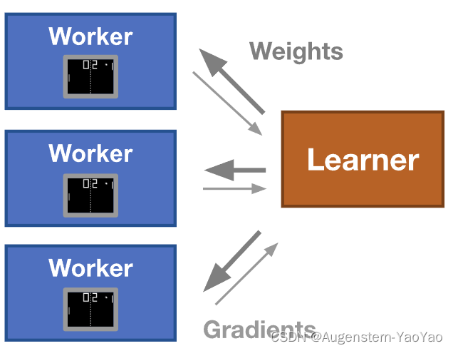
在此示例中将使用 Gymnasium 训练一个非常简单的神经网络来玩 Pong 游戏。从高层次来看,将使用多个 Ray actors 同时获取模拟展开和计算梯度。然后将集中这些梯度并更新神经网络。更新后的神经网络将传回到每个 Ray actor 以进行更多的梯度计算。
环境配置
在RayRLlib环境的基础上,还需要安装:
pip install gymnasium[atari] gym==0.26.2
pip install pyyaml
pip install -U "ray[tune]"
pip install gym[accept-rom-license]
目前,在一台具有64个物理核心的大型机器上,使用大小为1的批次计算更新大约需要1秒,大小为10的批次大约需要2.5秒。大小为60的批次大约需要3秒。在一个具有11个节点的集群上,每个节点有18个物理核心,大小为300的批次大约需要10秒。这些时间取决于并行计算时各个计算设备所需的时间,而这又取决于策略的表现。例如,一个非常糟糕的策略会很快失败。随着策略的学习,可以预期这些数字会增加。
代码实现
import numpy as np
import os
import ray
import time

import gymnasium as gym
定义几个使用的超参数:
H = 200  # The number of hidden layer neurons.
gamma = 0.99  # The discount factor for reward.
decay_rate = 0.99  # The decay factor for RMSProp leaky sum of grad^2.
D = 80 * 80  # The input dimensionality: 80x80 grid.
learning_rate = 1e-4  # Magnitude of the update.
首先定义几个辅助函数:
- 预处理:preprocess 函数将原始的 210x160x3 uint8 帧预处理为一个一维的 6400 浮点向量。
- 奖励处理:process_rewards 函数将计算一个折扣奖励。该公式表明,采样的行动的“价值”是随后所有奖励的加权和,但后面的奖励指数级地不那么重要。
- 回合:rollout 函数玩整个乒乓球游戏(直到电脑或强化学习代理输了)。
def preprocess(img):
    # Crop the image.
    img = img[35:195]
    # Downsample by factor of 2.
    img = img[::2, ::2, 0]
    # Erase background (background type 1).
    img[img == 144] = 0
    # Erase background (background type 2).
    img[img == 109] = 0
    # Set everything else (paddles, ball) to 1.
    img[img != 0] = 1
    return img.astype(np.float).ravel()


def process_rewards(r):
    """Compute discounted reward from a vector of rewards."""
    discounted_r = np.zeros_like(r)
    running_add = 0
    for t in reversed(range(0, r.size)):
        # Reset the sum, since this was a game boundary (pong specific!).
        if r[t] != 0:
            running_add = 0
        running_add = running_add * gamma + r[t]
        discounted_r[t] = running_add
    return discounted_r


def rollout(model, env):
    """Evaluates  env and model until the env returns "Terminated" or "Truncated".

    Returns:
        xs: A list of observations
        hs: A list of model hidden states per observation
        dlogps: A list of gradients
        drs: A list of rewards.

    """
    # Reset the game.
    observation, info = env.reset()
    # Note that prev_x is used in computing the difference frame.
    prev_x = None
    xs, hs, dlogps, drs = [], [], [], []
    terminated = truncated = False
    while not terminated and not truncated:
        cur_x = preprocess(observation)
        x = cur_x - prev_x if prev_x is not None else np.zeros(D)
        prev_x = cur_x

        aprob, h = model.policy_forward(x)
        # Sample an action.
        action = 2 if np.random.uniform() < aprob else 3

        # The observation.
        xs.append(x)
        # The hidden state.
        hs.append(h)
        y = 1 if action == 2 else 0  # A "fake label".
        # The gradient that encourages the action that was taken to be
        # taken (see http://cs231n.github.io/neural-networks-2/#losses if
        # confused).
        dlogps.append(y - aprob)

        observation, reward, terminated, truncated, info = env.step(action)

        # Record reward (has to be done after we call step() to get reward
        # for previous action).
        drs.append(reward)
    return xs, hs, dlogps, drs
定义策略神经网络
这里,神经网络被用来定义打乒乓球的“策略”(即,在给定状态下选择一个行动的函数)。
为了在 NumPy 中实现神经网络,需要提供帮助函数来计算更新和计算神经网络的输出,给定一个输入,我们的情况下是一个观察。
class Model(object):
    """This class holds the neural network weights."""

    def __init__(self):
        self.weights = {}
        self.weights["W1"] = np.random.randn(H, D) / np.sqrt(D)
        self.weights["W2"] = np.random.randn(H) / np.sqrt(H)

    def policy_forward(self, x):
        h = np.dot(self.weights["W1"], x)
        h[h < 0] = 0  # ReLU nonlinearity.
        logp = np.dot(self.weights["W2"], h)
        # Softmax
        p = 1.0 / (1.0 + np.exp(-logp))
        # Return probability of taking action 2, and hidden state.
        return p, h

    def policy_backward(self, eph, epx, epdlogp):
        """Backward pass to calculate gradients.

        Arguments:
            eph: Array of intermediate hidden states.
            epx: Array of experiences (observations).
            epdlogp: Array of logps (output of last layer before softmax).

        """
        dW2 = np.dot(eph.T, epdlogp).ravel()
        dh = np.outer(epdlogp, self.weights["W2"])
        # Backprop relu.
        dh[eph <= 0] = 0
        dW1 = np.dot(dh.T, epx)
        return {"W1": dW1, "W2": dW2}

    def update(self, grad_buffer, rmsprop_cache, lr, decay):
        """Applies the gradients to the model parameters with RMSProp."""
        for k, v in self.weights.items():
            g = grad_buffer[k]
            rmsprop_cache[k] = decay * rmsprop_cache[k] + (1 - decay) * g ** 2
            self.weights[k] += lr * g / (np.sqrt(rmsprop_cache[k]) + 1e-5)


def zero_grads(grad_buffer):
    """Reset the batch gradient buffer."""
    for k, v in grad_buffer.items():
        grad_buffer[k] = np.zeros_like(v)
并行化梯度
定义一个 Ray actor,它负责接受一个模型和一个环境,并执行回合 + 计算梯度更新的任务。
os.environ["OMP_NUM_THREADS"] = "1"
# 强制 OpenMP 使用一个单线程,这是为了防止多个 actor 之间发生竞争。

# 告诉 numpy 只使用一个核心。如果我们不这样做,每个 actor 可能会尝试使用所有核心,结果会导致争用,从而无法加速串行版本。
# 请注意,如果 numpy 正在使用 OpenBLAS,则需要设置 OPENBLAS_NUM_THREADS=1,并且您可能需要在命令行中执行此操作(以便在导入 numpy 之前发生)。
os.environ["MKL_NUM_THREADS"] = "1"

ray.init()

@ray.remote
class RolloutWorker(object):
    def __init__(self):
        self.env = gym.make("GymV26Environment-v0", env_id="ALE/Pong-v5")

    def compute_gradient(self, model):
        # Compute a simulation episode.
        xs, hs, dlogps, drs = rollout(model, self.env)
        reward_sum = sum(drs)
        # Vectorize the arrays.
        epx = np.vstack(xs)
        eph = np.vstack(hs)
        epdlogp = np.vstack(dlogps)
        epr = np.vstack(drs)

        # Compute the discounted reward backward through time.
        discounted_epr = process_rewards(epr)
        # Standardize the rewards to be unit normal (helps control the gradient
        # estimator variance).
        discounted_epr -= np.mean(discounted_epr)
        discounted_epr /= np.std(discounted_epr)
        # Modulate the gradient with advantage (the policy gradient magic
        # happens right here).
        epdlogp *= discounted_epr
        return model.policy_backward(eph, epx, epdlogp), reward_sum
上述代码通过 Ray 框架创建了 batch_size 个 RolloutWorker 远程对象,这些对象将并行计算梯度。这里 batch_size 设定了并行度。这里的并行计算与线程并行不完全相同,Ray 使用 Actor 模型并行地执行这些远程对象。实际上,Ray 可以根据可用资源(如 CPU 核心或 GPU)智能地调度这些远程对象,从而实现分布式计算。
因此,在这个例子中,可以将 batch_size 视为并行度的指示。增加 batch_size 的值会增加并行执行的 RolloutWorker 数量,从而增加并行计算能力。
训练
这个例子很容易并行化,因为网络可以并行地玩十场(如果batch_size=10)比赛,并且游戏之间不需要共享信息。在循环中,网络不断地玩乒乓球游戏,并记录每场游戏的梯度。每十场游戏,这些梯度被组合在一起,用于更新网络。
iterations = 5   # 迭代回合为500次时,达到-16的奖励值
batch_size = 20  # batch_size 设定了并行度
model = Model()
# 代码创建了 batch_size 个 RolloutWorker 对象:
actors = [RolloutWorker.remote() for _ in range(batch_size)]

running_reward = None
# "Xavier" initialization.
# Update buffers that add up gradients over a batch.
grad_buffer = {k: np.zeros_like(v) for k, v in model.weights.items()}
# Update the rmsprop memory.
rmsprop_cache = {k: np.zeros_like(v) for k, v in model.weights.items()}

for i in range(1, 1 + iterations):
    model_id = ray.put(model)
    gradient_ids = []
    # Launch tasks to compute gradients from multiple rollouts in parallel.
    start_time = time.time()
    # 在训练循环中,这些 RolloutWorker 对象会并行计算梯度:
    gradient_ids = [actor.compute_gradient.remote(model_id) for actor in actors]
    for batch in range(batch_size):
        [grad_id], gradient_ids = ray.wait(gradient_ids)
        grad, reward_sum = ray.get(grad_id)
        # Accumulate the gradient over batch.
        for k in model.weights:
            grad_buffer[k] += grad[k]
        running_reward = (
            reward_sum
            if running_reward is None
            else running_reward * 0.99 + reward_sum * 0.01
        )
    end_time = time.time()
    print(
        "Batch {} computed {} rollouts in {} seconds, "
        "running mean is {}".format(
            i, batch_size, end_time - start_time, running_reward
        )
    )
    model.update(grad_buffer, rmsprop_cache, learning_rate, decay_rate)
    zero_grads(grad_buffer)

    # 保存模型权重
for k, v in model.weights.items():
    np.save(f"{k}_weights.npy", v)