引言
机器人的动力学方程通常可以通过牛顿-欧拉公式或拉格朗日动力学公式得到。
关于机器人动力学是什么,可以参考Robitics公众号的这一系列文章干货 | 机械臂的动力学(二):拉格朗日法;或者在CSDN上找,资料很多,如机器人动力学——拉格朗日法
——简单来说,牛顿-欧拉公式通过力学分析得到运动方程,而拉格朗日动力学公式从能量角度得到运动方程。
Q:什么是运动方程?
A:百度上的解答为:“运动方程是描述结构中力与位移(包括速度和加速度)关系的数学表达式。现在的各种模型,通常为多输入多输出形式,一种比较合适的建模方式是通过状态空间进行建模。
在分析时,常常以广义位置【位移、角度】、广义速度【速度,角速度】为状态向量 x x x; x ˙ \dot{x} x˙自然而然牵扯到广义加速度【加速度,角加速度】;
此外,这类建模中输入向量 u u u通常为力矩【移动副】或者扭矩【转动副】
因此,运动方程常常是广义加速度、广义速度、广义位置和输入向量之间的关系等式组
本文将简单介绍拉格朗日动力学建模过程,并以一阶倒立摆建模过程为例,手推运动方程,并在matlab借助代码验证该过程。
拉格朗日方程
拉格朗日量 L \mathcal{L} L可以用以下公式表示:
L ( q , q ˙ ) = T ( q , q ˙ ) − V ( q ) \mathcal{L}(\mathrm{q}, \dot{\mathrm{q}})=\mathcal{T}(\mathrm{q}, \dot{\mathrm{q}})-\mathcal{V}(\mathrm{q}) L(q,q˙)=T(q,q˙)−V(q),其中 T \mathcal{T} T为系统动能、 V \mathcal{V} V为系统势能。
哈狗恩朗日公式法可以用以下公式表示
d d t ( ∂ L ∂ q ˙ j ) − ∂ L ∂ q j = f \begin{array}{l} \frac{d}{d t}\left(\frac{\partial\mathcal{L}}{\partial \dot{q}_{j}}\right)-\frac{\partial\mathcal{L}}{\partial q_{j}}=f \end{array} dtd(∂q˙j∂L)−∂qj∂L=f
这个方程也称为含外力的欧拉-拉格朗日方程(在标准形式的欧拉-拉格朗日方程中,外力 f f f 等于零)
Q:零势能面怎么选择呢?是以水平方向为零重力势能吗?
——零势能面不影响最终答案,相当于势能 V \mathcal V V加了一个不随时间变化的常数
此外【这部分内容笔者并没有找到太好的资料,有待补充,同时也欢迎大家在评论区分享自己找到的的资料】
根据系统的串并联结构,可划分第一类拉格朗日方程和第二类拉格朗日方程
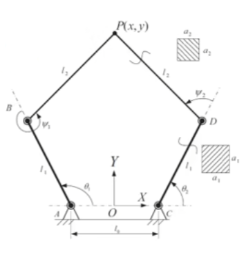
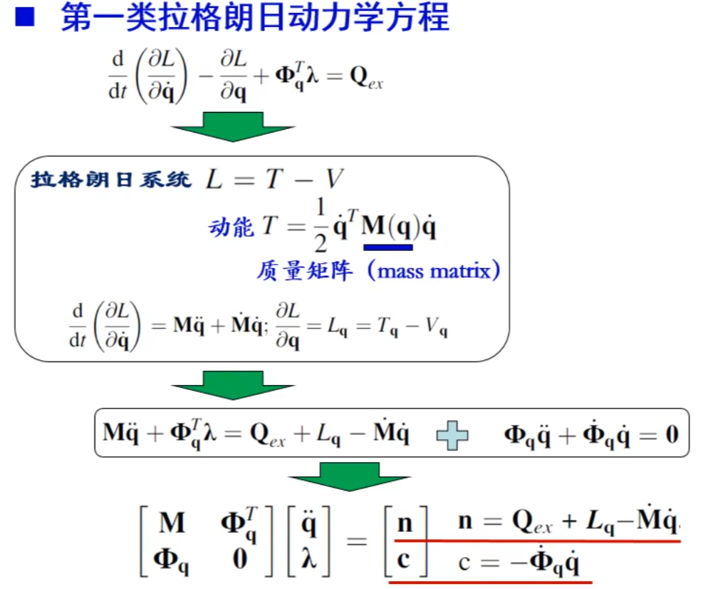
- 第一类: d d t ( ∂ L ∂ q ˙ ) − ∂ L ∂ q + Φ q T λ = Q e x \frac{\mathrm{d}}{\mathrm{d} t}\left(\frac{\partial \mathcal{L}}{\partial \dot{\mathbf{q}}}\right)-\frac{\partial\mathcal{L}}{\partial \mathbf{q}}+\boldsymbol{\Phi}_{\mathbf{q}}^{T} \lambda=\mathbf{Q}_{e x} dtd(∂q˙∂L)−∂q∂L+ΦqTλ=Qex,适用于闭环结构,即并联机构
如双足模型中常用的五连杆模型或者七连杆模型
如图所示的P点不仅会被A影响,也会被C影响
- 第二类: d d t ( ∂ L ∂ q ˙ ) − ∂ L ∂ q = Q e x \frac{\mathrm{d}}{\mathrm{d} t}\left(\frac{\partial \mathcal{L}}{\partial \dot{\mathbf{q}}}\right)-\frac{\partial \mathcal{L}}{\partial \mathbf{q}}=\mathbf{Q}_{e x} dtd(∂q˙∂L)−∂q∂L=Qex适用于开环结构,即串联机构,本文讨论的就是串联机构
一阶倒立摆的建模
物理模型
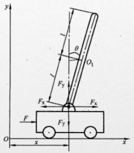
变量声明
| 物理量 | 符号 |
|---|---|
| 滑块质量 | M M M |
| 摆杆质量 | m m m |
| 摆杆转动轴心到杆质心长度【半杆长】 | l l l |
| 摆杆在转轴处转动惯量 | J J J |
| 小车受到外力 | F F F |
| 小车位置 | x x x |
| 摆杆与竖直方向夹角【本文顺时针为正】 | θ \theta θ |
力学分析
对滑块分析: M x ¨ = F − F x (1) \begin{array}{l} M{\ddot{x}}=F - F_{x}\end{array}\tag{1} Mx¨=F−Fx(1)
对杆分析:
{ x向: F x = m d 2 d t 2 ( x + l sin θ ) y向: F y − m g = m d 2 d t 2 ( l cos θ ) 力矩: F y l sin θ − F x l cos θ = J θ ¨ (2) \left\{\begin{array}{l} \text { x向: } F_{x}=m \frac{d^{2}}{dt^2}\left(x+l \sin \theta\right) \\\\ \text { y向: } F_{y}-m g=m \frac{d^{2}}{d t^{2}}\left(l \cos \theta\right) \\\\ \text {力矩: } {F_{y}l\sin \theta}-{F_{x} l\cos \theta}=J \ddot{\theta} \end{array}\tag{2}\right. ⎩
⎨
⎧ x向: Fx=mdt2d2(x+lsinθ) y向: Fy−mg=mdt2d2(lcosθ)力矩: Fylsinθ−Fxlcosθ=Jθ¨(2)
公式推导
x 向 → F x = m x ¨ + m l ( cos θ ⋅ θ ¨ − sin θ ⋅ θ ˙ 2 ) (3) \begin{array}{l} x向\rightarrow F_{x} =m \ddot{x}+m l \left( \cos\theta\cdot\ddot{\theta}-\sin\theta\cdot \dot{\theta}^{2}\right)\end{array}\tag{3} x向→Fx=mx¨+ml(cosθ⋅θ¨−sinθ⋅θ˙2)(3)
y 向 → F y = m g − m l [ sin θ ⋅ θ ¨ + cos θ ⋅ θ ˙ 2 ] (4) \begin{array}{l} y向\rightarrow F_{y} =m g-m l \left[\sin\theta\cdot\ddot{\theta}+\cos \theta \cdot \dot{\theta}^{2}\right]\end{array}\tag{4} y向→Fy=mg−ml[sinθ⋅θ¨+cosθ⋅θ˙2](4)
带入力矩式,
( m g l sin θ − m l 2 sin 2 θ ⋅ θ ¨ − m l 2 sin θ cos θ ⋅ θ ˙ 2 ) − ( m l cos θ ⋅ x ¨ + m l 2 cos 2 θ ⋅ θ ¨ − m l 2 cos θ sin θ ⋅ θ ˙ 2 ) = J θ ¨ (5) \begin{array}{l} ({m g l \sin \theta}-{m l^2 \sin^2 \theta\cdot \ddot{\theta}}-{m l^2 \sin \theta \cos \theta\cdot \dot{\theta}^{2}})-({m l \cos\theta \cdot\ddot{x}}+{m l^{2} \cos^2 \theta\cdot\ddot{\theta}}-{m l^2 \cos \theta \sin\theta\cdot \dot{\theta}^{2}})=J \ddot{\theta} \tag{5} \end{array} (mglsinθ−ml2sin2θ⋅θ¨−ml2sinθcosθ⋅θ˙2)−(mlcosθ⋅x¨+ml2cos2θ⋅θ¨−ml2cosθsinθ⋅θ˙2)=Jθ¨(5)
运行结果
利用 sin 2 θ + cos 2 θ = 1 \sin^2\theta+\cos^2\theta=1 sin2θ+cos2θ=1,有:
m g l sin θ − m l cos θ ⋅ x ¨ = ( J + m l 2 ) ⋅ θ ¨ (6) \begin{array}{l} {m g l \sin \theta}-{m l \cos\theta} \cdot\ddot{x}=(J+{m l^2 }) \cdot\ddot{\theta} \tag{6} \end{array} mglsinθ−mlcosθ⋅x¨=(J+ml2)⋅θ¨(6)
另外,将(3)代入(1),有
− m l sin θ ⋅ θ ˙ 2 + m l cos θ ⋅ θ ¨ + ( M + m ) ⋅ x ¨ = F (7) \begin{array}{l}\\ -ml\sin\theta\cdot \dot{\theta}^{2}+m l \cos\theta\cdot\ddot{\theta}+(M + m)\cdot{\ddot{x}}=F\tag{7} \end{array} −mlsinθ⋅θ˙2+mlcosθ⋅θ¨+(M+m)⋅x¨=F(7)
拉格朗日法建模
系统动能由滑块动能 T 1 T_1 T1和摆杆动能 T 2 T_2 T2构成
滑块纯滑动
T 1 = 1 2 ∗ M ∗ v 2 , v = d d t x T_1 = \frac{1}{2}*M*v^2, v=\frac{d}{dt}x T1=21∗M∗v2,v=dtdx
摆杆滑动+摆动
T 2 = 1 2 ∗ m ∗ v 2 , v = d d t p T_2 = \frac{1}{2}*m*v^2, v=\frac{d}{dt}p T2=21∗m∗v2,v=dtdp
其中 p p p点坐标为 p = ( s + l 2 sin θ , l 2 cos θ ) p=(s+\frac{l}{2}\sin\theta,\frac{l}{2}\cos\theta) p=(s+2lsinθ,2lcosθ)
重力势能
V = m ∗ g ∗ 1 / 2 ∗ l ∗ cos θ V=m*g*1/2*l*\cos\theta V=m∗g∗1/2∗l∗cosθ
构造matlab代码
clear all
syms g M m l s(t) J theta(t) F(t)

T1 = 1/2*M*diff(s,t)^2;
T2 = 1/2*J*diff(theta,t)^2 + 1/2*m*(diff(s+1/2*l*sin(theta),t)^2 + diff(1/2*l*cos(theta),t)^2);
V = m*g*1/2*l*cos(theta);
L = T1 +T2 - V;
eqn = functionalDerivative(L,[s;theta]) == [-F;0]
eqn = simplify(eqn)
【若报错注意看看是不是下载matlab时没有下载对应组件,按照当时的Matlab安装流程重新安装】
运行结果
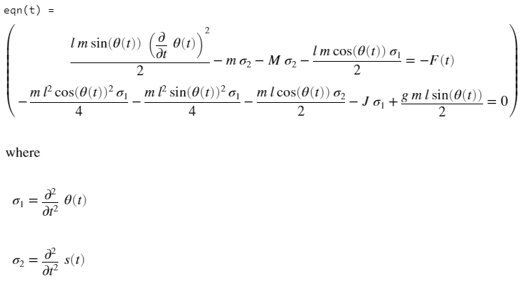
附:上文的(6) (7)
{ m g l sin θ − m l cos θ ⋅ x ¨ = ( J + m l 2 ) ⋅ θ ¨ − m l sin θ ⋅ θ ˙ 2 + m l cos θ ⋅ θ ¨ + ( M + m ) ⋅ x ¨ = F \left\{\begin{array}{l} {m g l \sin \theta}-{m l \cos\theta} \cdot\ddot{x}=(J+{m l^2 }) \cdot\ddot{\theta} \\\\ -ml\sin\theta\cdot \dot{\theta}^{2}+m l \cos\theta\cdot\ddot{\theta}+(M + m)\cdot{\ddot{x}}=F \end{array}\right. ⎩
⎨
⎧mglsinθ−mlcosθ⋅x¨=(J+ml2)⋅θ¨−mlsinθ⋅θ˙2+mlcosθ⋅θ¨+(M+m)⋅x¨=F
二者表达等价
至此,拉格朗日建模过程已经实现,以下是一个完整的例子。
拉格朗日法+设置初值求系统中变量
如题所示为弹簧-滑块模型,表面光滑
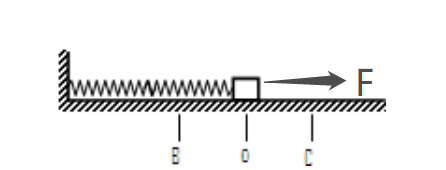
- 设置初值:若弹簧一开始有伸长量 d x 0 dx_0 dx0或者物块一开始有速度 v 0 v_0 v0,则可以求出物块距离初值位置随时间的表达式
设弹簧原长为 x 0 x_0 x0【不重要】,在Matlab中可根据初始伸长量和速度求得x的表达式【此时的x事实上是dx,代表弹簧伸长量】
clear all
x0 = 10
syms m k x(t)
T = 1/2*m*diff((x+x0), t)^2;
V = 1/2*k*x^2;
L = T - V;
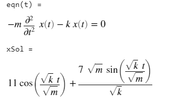
eqn = functionalDerivative(L, x) == 0
assume(m, "positive")
assume(k, "positive")
Dx(t) = diff(x(t), t);
xSol = dsolve(eqn, [x(0) == 11, Dx(0) == 7])
- 运行结果如下
- 验证环节
知识储备不足,不会验证。。。
能想到的方法就是利用能量关系列出与x有关的方程式并求解,实现过程与此方法完全一致。
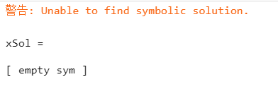
我还没摸清楚这种方法在多维变量(多输入多输出【尤其是多输入】)时怎么使用,它的求解思路以及原理尚不清楚,有待探究
多输入时,报错如下:
写在后面
- Matlab中的
functionalDerivative函数应该只是一个求微分方程的函数,然后 拉格朗日动力学方程 是写成了微分方程形式的函数,因此可以用这个函数求解 - 这个函数的泛用性应该很强
参考文献
本文的部分方法及代码来自B站视频教程LQR倒立摆 从建模到控制 零基础都能复现,推荐观看!