Finite Markov Decision Processes

MDPs are a classical formalization of sequential decision making. MDPs are a mathmatically idealized form of the reinforcement learning problem for which precise theoretical statements can be made. As in all of artificial intelligence, there is a tension between breadth of applicability and mathematical tractability.

1. The Agent-Environment Interface

The learner and decision maker is called the agent.
The thing it interacts with, comprising everything outside the agent, is called the environment.
(We uses the terms agent, environment, and action instead of the engineers’ terms controller, controlled system(or plant), and control signal because they are meaningful to a wider audience.)

In particular, the boundary between agent and environment is typically not the same as the physical boudary of robot’s or animal body. The general rule we follow is that anything that cannot be changed arbitrarily by the agent is considered to be outside of it and thus part of its environment.

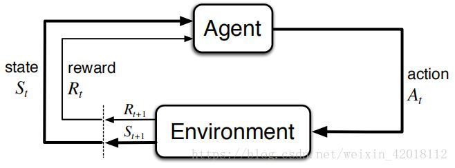
Figure 1: The agent-environment interaction in a Markov decision process.

The probabilities given by the four-argument function $p$ completely characterize the dynamics of a finite MDP:

$$p(s^{'},r\mid s,a)\doteq \mathrm{Pr}\left \{ S_{t}=s^{'},R_{t}=r\mid S_{t-1}=s,A_{t-1}=a \right \}$$
From it, we can compute anything else one might want to know about the environment.
For example:

• the state-transition probabilities
• the expected rewards for state-action pairs
• the expected rewards for state-action-next-state triples

The MDP framework is a considerable abstraction of the problem of goal-directed learning from interaction. Any problem of learning goal-directed behevior can be reduced to three signals passing back and forth between an agent and its environment: one signal to represent the choices made by the agent (the actions), one signal to represent the basis on which choices are made (the states), and one signal to defineteh agent’s goal (the rewards).

2. Goals and Rewards

That all of what we mean by goals and purposes can be well thought of as the maximization of othe expected value of the cumulative sum of a receive scalar signal (called reward).

It is thus critical that the rewards we set up truly indicate what we want accomplished. In paricular, the reward signal is not the place to impart to the agent prior knowledge about how to achieve what we want it to do.

3. Returns and Episodes

In general, we seek to maximize the expected return, where the return, denoted $G_{t}$, is defined as some specific function of the reward sequence.

$$G_{t}\doteq R_{t+1}+\gamma R_{t+2}+\gamma ^{2}R_{t+3}+\cdots =\sum_{k=0}^{\infty}\gamma ^{k}R_{t+k+1}$$
The discount rate determines the present value of future rewards: a reward received k time steps in the future is worth only $\gamma^{k-1}$ times what it would be worth if it were reveived immediately.
If $\gamma < 1$, the infibite sum above have a finite value as long as the reward sequence ${R_{k}}$ bounded.
If $\gamma=0$, the agent is “myopic” in being concerned only with maximizing immediate rewards.

Returns at successive time steps are related to each other in a way that is important for the theory and algorithms of reinforcement learning:

$$G_{t}\doteq R_{t+1}+\gamma R_{t+2}+\gamma ^{2}R_{t+3}+\cdots =R_{t+1}+\gamma (R_{t+2}+\gamma R_{t+3}+\gamma ^{2}R_{t+4}+\cdots)=R_{t+1}+\gamma G_{t+1}$$

5. Policies and Value Functions

Almost all reinforcement learning algorithms invlove estimating value functions—functions of states (or of state-action pairs) that esimate how good it is for the agent to be in a given state (or how good it is to perform a given action in a given state).

Formally, a policy is a mapping from states to probabilities of selecting each possible action.

$$\pi(a\mid s)=\mathrm{Pr}(A=a\mid S=s)$$

The value of a state $s$ under a policy $\pi$, denoted $v_{\pi}(s)$, is the expected return when starting in $s$ and following $\pi$ thereafter.
state-value function for policy $\pi$:

$$v_{\pi}(s)\doteq \mathbb{E}_{\pi}[G_{t}\mid S_{t}=s]=\mathbb{E}_{\pi}\left [ \sum_{k=0}^{\infty}\gamma^{k}R_{t+k+1}\mid S_{t}=s \right ]$$

Similarly, we difine the value of taking action $a$ in state $s$ under a policy $\pi$, denoted $q_{\pi}(s,a)$, as the expected return starting from $s$, taking the action $a$, and thereafter following policy $\pi$.
action-value function for policy $\pi$:

$$q_{\pi}(s,a)\doteq \mathbb{E}_{\pi}[G_{t}\mid S_{t}=s,A_{t}=a]=\mathbb{E}_{\pi}\left [ \sum_{k=0}^{\infty}\gamma^{k}R_{t+k+1}\mid S_{t}=s,A_{t}=a \right ]$$

For any policy $\pi$ and any state $s$, the following consistency condition holds between the value of $s$ and the value of its possible successor states:

$$v_{\pi}(s)\doteq \mathbb{E}_{\pi}[G_{t}\mid S_{t}=s]=\mathbb{E}_{\pi}[R_{t+1}+\gamma G_{t+1}\mid S_{t}=s]$$
$$=\sum_{a}\pi(a\mid s)\sum_{s^{'}}\sum_{r}p(s^{'},r\mid s,a)\left [ r+\gamma\mathbb{E}_{\pi}[G_{t+1}\mid S_{t+1}=s^{'}] \right ]$$
$$=\sum_{a}\pi(a\mid s)\sum_{s^{'},r}p(s^{'},r\mid s,a)\left [ r+\gamma v_{\pi}(s^{'})] \right ]$$
Equation above is the Bellman equation for $v_{\pi}$. It expresses a relationship between the value of a state and the values of its successor states.
A fundamental property of value function used throughout RL is that they satisfy recursive relationships similar to that which we have already established for the return.