[Matlab]频率f，角频率Ω和数字频率w的物理含义

需要结合

http://anony3721.blog.163.com/blog/static/51197420111129503233/

或者

https://blog.csdn.net/xiaoyanwin/article/details/15420707

食用。

%信号处理中的各种频率
%freqs.m
%MatlabR2015b
%2018年6月4日 09:46:34

clear;
close all;
clc;
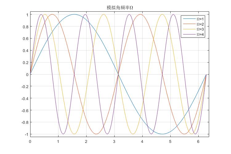
%模拟角频率 Omega: rad/s
%物理意义:在2*pi的时间段里面包含的y=sin(Omega*t)正弦信号的个数
t = 0:pi/100:2*pi;
for Omega = 1:4
    y(:,Omega) = sin(Omega*t);
    str{Omega} = ['\Omega=',num2str(Omega)];
end

figure('Position',[ 300 300 750 500]);
h = plot(t',y);
title('模拟角频率\Omega');
axis([0,2*pi+0.1 -1.05 1.05 ]);
legend(h,str);
grid on;

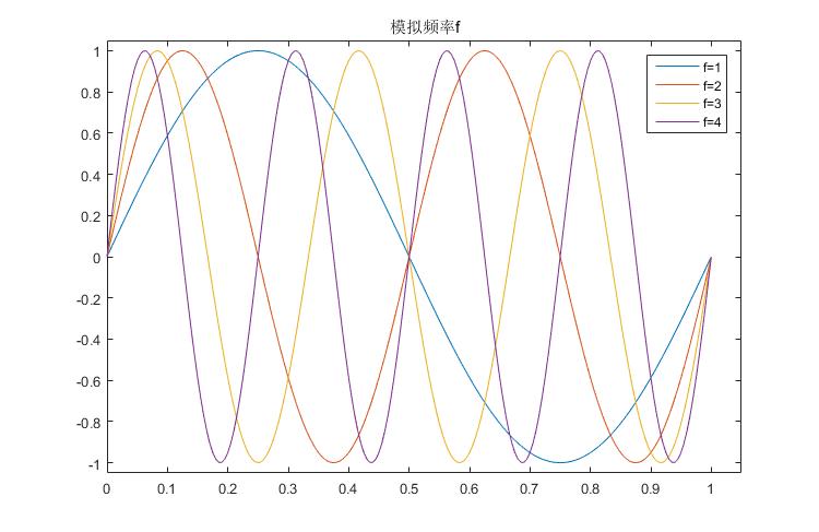
%模拟频率f: hz
%物理意义:在1s的时间段内含有f个y=sin(f*t)完整周期的波形信号
clear;
t = 0:1/200:1;
for f = 1:4
    y(:,f) = sin(2*pi*f*t);
    str{f} = ['f=',num2str(f)];
end
figure('Position',[ 300 300 750 500]);
h = plot(t',y);
axis([0,1.05 -1.05 1.05 ]);
title('模拟频率f');
legend(h,str);


%数字频率w(归一化过的)
%1.数字频率必须跟采样周期Ts结合在一起才有意义
%2.数字频率是从单位圆上N点等间隔采样而来的，这个N就是数字周期
%3.数字频率和数字周期之间的关系 w = k*2*pi/N
%4.数字频率w和模拟频率之间的关系：
% w = Omega*Ts = Omega/Fs,使用Fs归一化后的频率
clear;
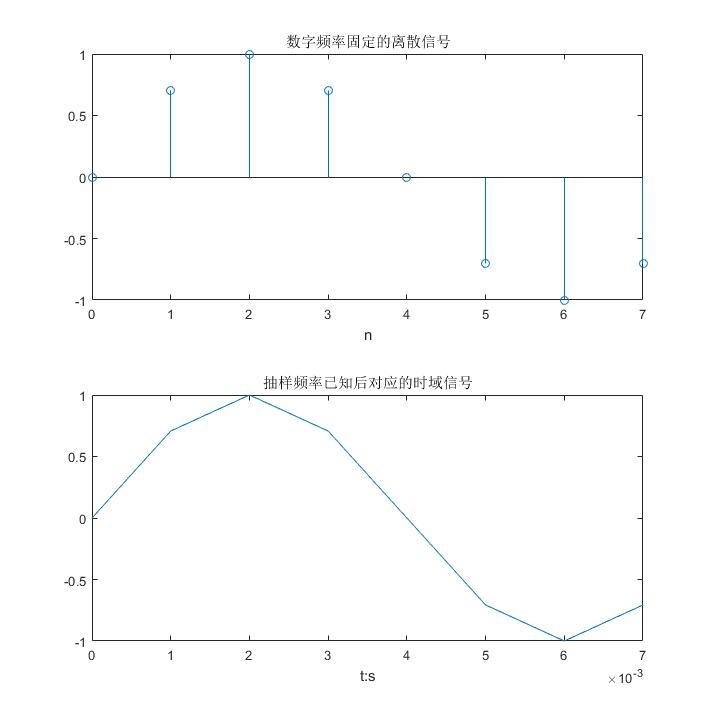
w = pi/4;
N = 2*pi/w;  %N = 8
n = 0:N-1;
x = sin(n*w);  %生成离散序列
figure('Position',[ 300 300 750 500]);
subplot(2,1,1);
stem(n,x);
title('数字频率固定的离散信号');
xlabel('n');
Fs = 1000; %采样频率是1000Hz
Ts = 1/Fs;
t = n*Ts;%对应连续信号时刻
T = N*Ts;%模拟周期
f = w*Fs/(2*pi); %信号的真实频率
subplot(2,1,2);
plot(t,x);
xlabel('t:s');
title('抽样频率已知后对应的时域信号')
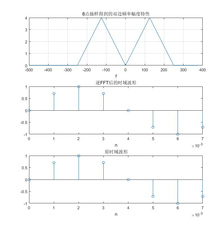
freq = n*Fs/N - Fs/2; %真正的双边谱频率量
X = fftshift(abs(fft(x))); %频谱搬移
x_ifft = ifft(fft(x));
figure('Position',[ 300 300 750 500]);
subplot(3,1,1);
plot(freq,X);
xlabel('f');
title('8点抽样得到的双边频率幅度特性');
grid on;
subplot(3,1,2);
stem(t,x_ifft);
title('逆FFT后的时域波形')
xlabel('n');
subplot(3,1,3);
stem(t,x);
title('原时域波形');
xlabel('n');

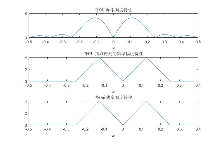
%fft补0
Nfft = 1024;
X_Nfft = fftshift(abs(fft(x,Nfft)));
freqNormalized = (-Nfft/2:Nfft/2-1)/Nfft;
figure('Position',[ 300 300 750 500]);
subplot(3,1,1);
plot(freqNormalized,X_Nfft);
title('补0后频率幅度特性');
xlabel('\omega');
subplot(3,1,2);
plot(freqNormalized(1:1024/8:end),X_Nfft(1:1024/8:end));
title('补0后抽取得到的频率幅度特性');
xlabel('\omega');
subplot(3,1,3);
plot(freq/Fs,X);
title('补0前频率幅度特性');
xlabel('\omega');



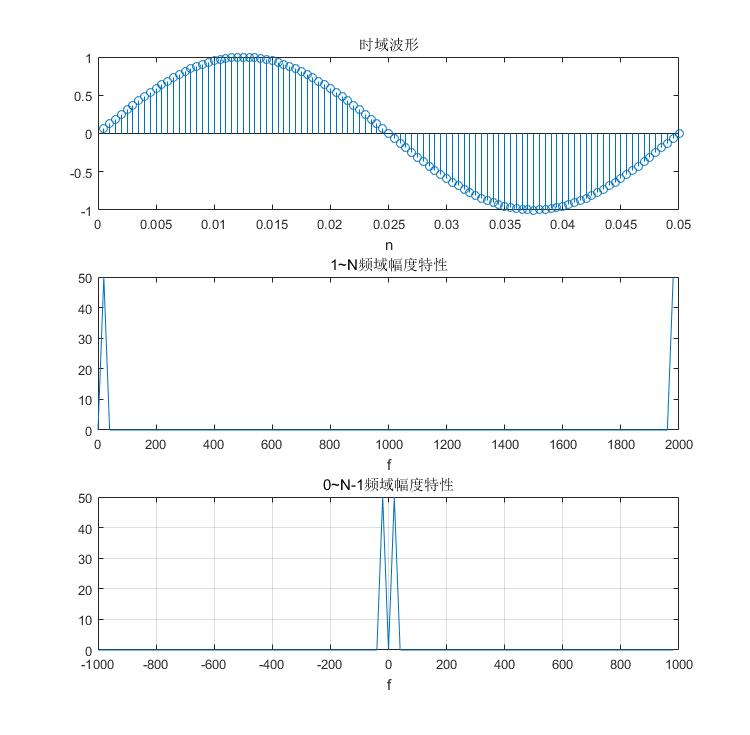
%0~N-1 和 1~N的区别
clear;
N = 100; %数字周期N
Fs = 2000; %采样频率
Ts = 1/Fs;%采样周期
n = 1:N;%频率点
w = 0.02*pi;
x = sin(w*n); %数字频率 w = 0.02*pi
t = n*Ts;
T = N*Ts;
f = w*Fs/(2*pi);
freq1 = n*Fs/N - Fs/N;
X = abs(fft(x));
figure('Position',[ 300 300 750 500]);
subplot(3,1,1);
stem(t,x);
xlabel('n');
title('时域波形')
subplot(3,1,2);
plot(freq1,X);
title('1~N频域幅度特性');
xlabel('f');
subplot(3,1,3);
freq =  (n-1)*Fs/N - Fs/2;
plot(freq,fftshift(abs(fft(x))));
title('0~N-1频域幅度特性');
xlabel('f');
grid on;