1. 项目介绍 + 环境配置
该项目源自ultralytics/yolov3
完整代码:https://github.com/WZMIAOMIAO/deep-learning-for-image-processing
霹老师YYDS ❤️
1.1 环境配置:
- Python 3.6或者3.7
- PyTorch 1.7.1 (注意:必须是1.6.0或以上,因为使用官方提供的混合精度训练1.6.0后才支持)
- pycocotools
- Linux:
pip install pycocotools - Windows:
pip install pycocotools-windows
- Linux:
- 更多环境配置信息,请查看
requirements.txt文件 - 最好使用GPU训练
1.2 文件结构:
  ├── cfg: 配置文件目录
  │    ├── hyp.yaml: 训练网络的相关超参数
  │    └── yolov3-spp.cfg: yolov3-spp网络结构配置
  │
  ├── data: 存储训练时数据集相关信息缓存
  │    └── pascal_voc_classes.json: pascal voc数据集标签
  │
  ├── runs: 保存训练过程中生成的所有tensorboard相关文件
  ├── build_utils: 搭建训练网络时使用到的工具
  │     ├── datasets.py: 数据读取以及预处理方法
  │     ├── img_utils.py: 部分图像处理方法
  │     ├── layers.py: 实现的一些基础层结构
  │     ├── parse_config.py: 解析yolov3-spp.cfg文件
  │     ├── torch_utils.py: 使用pytorch实现的一些工具
  │     └── utils.py: 训练网络过程中使用到的一些方法
  │
  ├── train_utils: 训练验证网络时使用到的工具(包括多GPU训练以及使用cocotools)
  ├── weights: 所有相关预训练权重(下面会给出百度云的下载地址)
  ├── model.py: 模型搭建文件
  ├── train.py: 针对单GPU或者CPU的用户使用
  ├── train_multi_GPU.py: 针对使用多GPU的用户使用
  ├── trans_voc2yolo.py: 将voc数据集标注信息(.xml)转为yolo标注格式(.txt)
  ├── calculate_dataset.py: 1)统计训练集和验证集的数据并生成相应.txt文件
  │                         2)创建data.data文件
  │                         3)根据yolov3-spp.cfg结合数据集类别数创建my_yolov3.cfg文件
  └── predict_test.py: 简易的预测脚本,使用训练好的权重进行预测测试
1.3 训练数据的准备以及目录结构
- 这里建议标注数据时直接生成YOLO格式的标签文件
.txt,推荐使用免费开源的标注软件 —— labelImg(支持YOLO格式) - 如果之前已经标注成pascal voc的
.xml格式了也没关系,通过脚本将voc转为yolo格式 - 测试图像时最好将图像缩放到32的倍数
- 标注好的数据集请按照以下目录结构进行摆放:
├── my_yolo_dataset 自定义数据集根目录
│         ├── train   训练集目录
│         │     ├── images  训练集图像目录
│         │     └── labels  训练集标签目录
│         └── val    验证集目录
│               ├── images  验证集图像目录
│               └── labels  验证集标签目录
1.4 利用标注好的数据集生成一系列相关准备文件
可参考原作者的教程
├── data 利用数据集生成的一系列相关准备文件目录
│    ├── my_train_data.txt:  该文件里存储的是所有训练图片的路径地址
│    ├── my_val_data.txt:  该文件里存储的是所有验证图片的路径地址
│    ├── my_data_label.names:  该文件里存储的是所有类别的名称,一个类别对应一行(这里会根据```.json```文件自动生成)
│    └── my_data.data:  该文件里记录的是类别数类别信息、train以及valid对应的txt文件
1.4.1 将VOC标注数据转为YOLO标注数据(如果你的数据已经是YOLO格式了,可跳过该步骤)
- 使用
trans_voc2yolo.py脚本进行转换,并在./data/文件夹下生成my_data_label.names标签文件, - 执行脚本前,需要根据自己的路径修改以下参数
# voc数据集根目录以及版本
voc_root = "./VOCdevkit"
voc_version = "VOC2012"

# 转换的训练集以及验证集对应txt文件,对应VOCdevkit/VOC2012/ImageSets/Main文件夹下的txt文件
train_txt = "train.txt"
val_txt = "val.txt"

# 转换后的文件保存目录
save_file_root = "/home/wz/my_project/my_yolo_dataset"

# label标签对应json文件
label_json_path = './data/pascal_voc_classes.json'
- 生成的
my_data_label.names标签文件格式如下
aeroplane
bicycle
bird
boat
bottle
bus
...
1.4.2 根据摆放好的数据集信息生成一系列相关准备文件
- 使用
calculate_dataset.py脚本生成my_train_data.txt文件my_val_data.txt文件my_data.data文件- 并生成新的
my_yolov3.cfg文件
- 执行脚本前,需要根据自己的路径修改以下参数
# 训练集的labels目录路径
train_annotation_dir = "./my_yolo_dataset/train/labels"
# 验证集的labels目录路径
val_annotation_dir = "./my_yolo_dataset/val/labels"
# 上一步生成的my_data_label.names文件路径(如果没有该文件,可以自己手动编辑一个txt文档,然后重命名为.names格式即可)
classes_label = "./data/my_data_label.names"
# 原始yolov3-spp.cfg网络结构配置文件
cfg_path = "./cfg/yolov3-spp.cfg"
1.5 预训练权重下载地址
下载后放入weights文件夹中:
yolov3-spp-ultralytics-416.pt: 链接: https://pan.baidu.com/s/1cK3USHKxDx-d5dONij52lA 密码: r3vmyolov3-spp-ultralytics-512.pt: 链接: https://pan.baidu.com/s/1k5yeTZZNv8Xqf0uBXnUK-g 密码: e3k1yolov3-spp-ultralytics-608.pt: 链接: https://pan.baidu.com/s/1GI8BA0wxeWMC0cjrC01G7Q 密码: ma3t
1.6 数据集
本例程使用的是PASCAL VOC2012数据集
Pascal VOC2012train/val数据集下载地址:http://host.robots.ox.ac.uk/pascal/VOC/voc2012/VOCtrainval_11-May-2012.tar
1.7 使用方法
- 确保提前准备好数据集
- 确保提前下载好对应预训练模型权重
- 若要使用单GPU训练或者使用CPU训练,直接使用train.py训练脚本
- 若要使用多GPU训练,使用
python -m torch.distributed.launch --nproc_per_node=8 --use_env train_multi_GPU.py指令,nproc_per_node参数为使用GPU数量
YOLOv3 SPP框架图
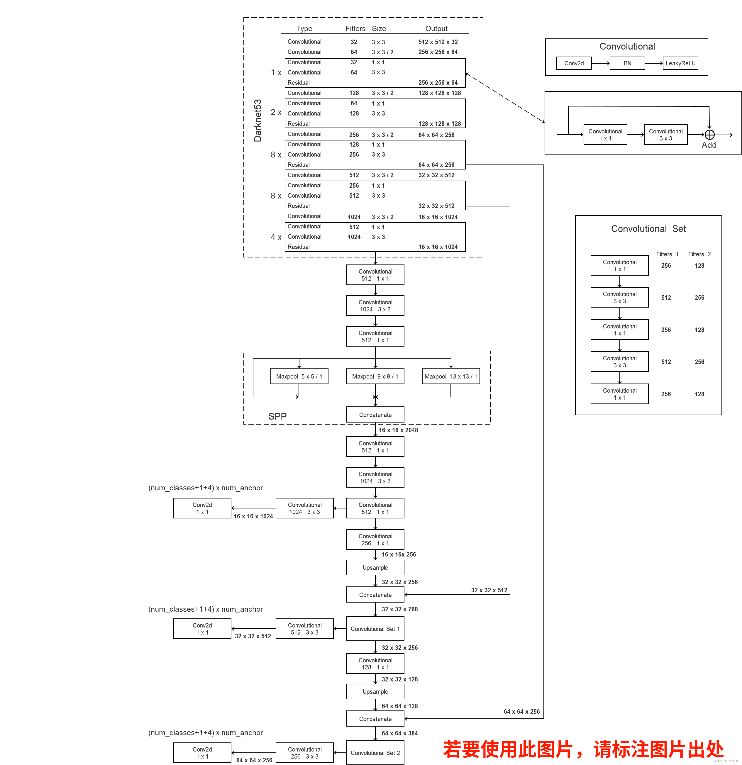
来源:https://www.bilibili.com/video/BV1t54y1C7ra?spm_id_from=333.999.0.0
2. 训练和预测脚本
2.1 训练脚本
import datetime
import argparse

import yaml
import torch.optim as optim
import torch.optim.lr_scheduler as lr_scheduler
from torch.utils.tensorboard import SummaryWriter

from models import *
from build_utils.datasets import *
from build_utils.utils import *
from train_utils import train_eval_utils as train_util
from train_utils import get_coco_api_from_dataset


def train(hyp):
    device = torch.device(opt.device if torch.cuda.is_available() else "cpu")
    print("Using {} device training.".format(device.type))

    wdir = "weights" + os.sep  # weights/dir  # os.sep是自适应分隔符
    best = wdir + "best.pt"
    results_file = "results{}.txt".format(datetime.datetime.now().strftime("%Y%m%d-%H%M%S"))

    cfg = opt.cfg
    data = opt.data
    epochs = opt.epochs
    batch_size = opt.batch_size
    """
        accumulate: 每训练xx张图片才会去更新它的权重
            如果我们的batch size因为显存的原因只能设置为4怎么办呢?
            通过这个公式我们发现,64/4=16,即每迭代16个batch才会更新一次参数

            通过这样的方式是有助于模型训练的!
    """
    accumulate = max(round(64 / batch_size), 1)  # accumulate n times before optimizer update (bs 64)
    weights = opt.weights  # initial training weights
    imgsz_train = opt.img_size
    imgsz_test = opt.img_size  # test image sizes
    multi_scale = opt.multi_scale

    # Image sizes
    # 图像要设置成32的倍数
    gs = 32  # (pixels) grid size
    # 这里会判断所指定的图像大小是否为32的倍数  math.fmod(a, b) == 0,判断a是否为b的整数倍
    assert math.fmod(imgsz_test, gs) == 0, "--img-size %g must be a %g-multiple" % (imgsz_test, gs)
    grid_min, grid_max = imgsz_test // gs, imgsz_test // gs
    if multi_scale:
        imgsz_min = opt.img_size // 1.5
        imgsz_max = opt.img_size // 0.667

        # 将给定的最大,最小输入尺寸向下调整到32的整数倍
        grid_min, grid_max = imgsz_min // gs, imgsz_max // gs
        imgsz_min, imgsz_max = int(grid_min * gs), int(grid_max * gs)
        imgsz_train = imgsz_max  # initialize with max size
        print("Using multi_scale training, image range[{}, {}]".format(imgsz_min, imgsz_max))

    # configure run
    # init_seeds()  # 初始化随机种子,保证结果可复现
    data_dict = parse_data_cfg(data)  # data/my_data.data这个文件
    train_path = data_dict["train"]  # data/my_train_data.txt:训练集中每个图片的路径
    test_path = data_dict["valid"]  # data/my_val_data.txt:验证集中每个图片的路径
    nc = 1 if opt.single_cls else int(data_dict["classes"])  # number of classes

    """
        根据超参数,调整cls_loss和obj_loss
            根据输入网络的类别个数和输入图片的指定大小
    """
    hyp["cls"] *= nc / 80  # update coco-tuned hyp['cls'] to current dataset
    hyp["obj"] *= imgsz_test / 320

    # Remove previous results
    for f in glob.glob(results_file):
        os.remove(f)

    # Initialize model
    model = Darknet(cfg).to(device)

    """
        + 从头开始训练的训练最差(不如只训练预测头)
        + 先进行预测头的训练,再进行除backbone的训练,比直接训练除backbone效果要好
    """
    # 是否冻结权重,只训练predictor的权重
    if opt.freeze_layers:
        # 索引减一对应的是predictor的索引,YOLOLayer并不是predictor
        output_layer_indices = [idx - 1 for idx, module in enumerate(model.module_list)
                                if isinstance(module, YOLOLayer)]
        # 冻结除predictor和YOLOLayer外的所有层
        freeze_layer_indeces = [x for x in range(len(model.module_list))
                                if (x not in output_layer_indices) and (x - 1 not in output_layer_indices)]

        # Freeze non-output layers
        # 总共训练3x2=6个parameters
        for idx in freeze_layer_indeces:
            for parameter in model.module_list[idx].parameters():
                # 对于需要冻结的层,不赋予其梯度attr
                parameter.requires_grad_(False)
    else:
        # 如果freeze_layer为False,默认仅训练除darknet53(backbone)之后的部分
        # 若要训练全部权重,删除以下代码
        darknet_end_layer = 74  # only yolov3spp cfg
        # Freeze darknet53 layers
        # 总共训练21x3+3x2=69个parameters
        for idx in range(darknet_end_layer + 1):  # [0, 74]
            for parameter in model.module_list[idx].parameters():
                parameter.requires_grad_(False)

    # optimizer
    pg = [p for p in model.parameters() if p.requires_grad]  # 将没有冻结的参数以list的形式传给pg(非冻结层的参数)
    optimizer = optim.SGD(pg,  # 将需要优化的参数(带有梯度的参数)传给优化器
                          lr=hyp["lr0"],
                          momentum=hyp["momentum"],
                          weight_decay=hyp["weight_decay"],
                          nesterov=True)

    # amp
    scaler = torch.cuda.amp.GradScaler() if opt.amp else None

    start_epoch = 0
    best_map = 0.0
    """
        权值文件中不仅仅保存了模型的参数,还保存了
        + 训练结果信息
        + 优化器信息
        + epoch信息
    """
    if weights.endswith(".pt") or weights.endswith(".pth"):
        ckpt = torch.load(weights, map_location=device)

        # load model
        try:
            # 检查权值文件是否完整
            ckpt["model"] = {

    k: v for k, v in ckpt["model"].items() if model.state_dict()[k].numel() == v.numel()}
            # 模型加载参数
            model.load_state_dict(ckpt["model"], strict=False)
        except KeyError as e:
            s = "%s is not compatible with %s. Specify --weights '' or specify a --cfg compatible with %s. " \
                "See https://github.com/ultralytics/yolov3/issues/657" % (opt.weights, opt.cfg, opt.weights)
            raise KeyError(s) from e

        # load optimizer
        if ckpt["optimizer"] is not None:
            optimizer.load_state_dict(ckpt["optimizer"])
            if "best_map" in ckpt.keys():
                best_map = ckpt["best_map"]

        # load results
        if ckpt.get("training_results") is not None:
            with open(results_file, "w") as file:
                file.write(ckpt["training_results"])  # write results.txt

        # epochs
        start_epoch = ckpt["epoch"] + 1
        if epochs < start_epoch:
            print('%s has been trained for %g epochs. Fine-tuning for %g additional epochs.' %
                  (opt.weights, ckpt['epoch'], epochs))
            epochs += ckpt['epoch']  # finetune additional epochs

        if opt.amp and "scaler" in ckpt:
            scaler.load_state_dict(ckpt["scaler"])

        del ckpt

    # Scheduler https://arxiv.org/pdf/1812.01187.pdf
    # 学习率更新策略 —— Cosine学习率
    lf = lambda x: ((1 + math.cos(x * math.pi / epochs)) / 2) * (1 - hyp["lrf"]) + hyp["lrf"]  # cosine
    scheduler = lr_scheduler.LambdaLR(optimizer, lr_lambda=lf)
    scheduler.last_epoch = start_epoch  # 指定从哪个epoch开始

    # 画学习率策略图(训练时不能画,建议使用Debug功能实现)
    # y = []
    # import matplotlib
    # matplotlib.use("TkAgg")
    # import matplotlib.pyplot as plt
    # plt.rcParams['font.sans-serif'] = ['Times New Roman']
    # for _ in range(epochs):
    #     scheduler.step()
    #     y.append(optimizer.param_groups[0]['lr'])
    # plt.plot(y, '.-', label='LambdaLR')
    # plt.xlabel('epoch')
    # plt.ylabel('LR')
    # plt.tight_layout()
    # plt.savefig('LR.png', dpi=300)

    # model.yolo_layers = model.module.yolo_layers

    # dataset
    # 训练集的图像尺寸指定为multi_scale_range中最大的尺寸
    train_dataset = LoadImagesAndLabels(train_path, imgsz_train, batch_size,
                                        augment=True,
                                        hyp=hyp,  # augmentation hyperparameters
                                        rect=opt.rect,  # rectangular training
                                        cache_images=opt.cache_images,
                                        single_cls=opt.single_cls)

    # 验证集的图像尺寸指定为img_size(512)
    val_dataset = LoadImagesAndLabels(test_path, imgsz_test, batch_size,
                                      hyp=hyp,
                                      rect=True,  # 将每个batch的图像调整到合适大小,可减少运算量(并不是512x512标准尺寸)
                                      cache_images=opt.cache_images,
                                      single_cls=opt.single_cls)

    # dataloader
    # 计算number of workers
    nw = min([os.cpu_count(), batch_size if batch_size > 1 else 0, 8])  # number of workers
    train_dataloader = torch.utils.data.DataLoader(train_dataset,
                                                   batch_size=batch_size,
                                                   num_workers=nw,
                                                   # Shuffle=True unless rectangular training is used
                                                   shuffle=not opt.rect,
                                                   pin_memory=True,
                                                   collate_fn=train_dataset.collate_fn)

    val_datasetloader = torch.utils.data.DataLoader(val_dataset,
                                                    batch_size=batch_size,
                                                    num_workers=nw,
                                                    pin_memory=True,
                                                    collate_fn=val_dataset.collate_fn)

    # Model parameters
    # 将下面3个参数添加到模型的变量中 —— 在计算Loss时会使用到
    model.nc = nc  # attach number of classes to model
    model.hyp = hyp  # attach hyperparameters to model
    model.gr = 1.0  # giou loss ratio (obj_loss = 1.0 or giou)
    # 计算每个类别的目标个数,并计算每个类别的比重
    # model.class_weights = labels_to_class_weights(train_dataset.labels, nc).to(device)  # attach class weights

    # start training
    # caching val_data when you have plenty of memory(RAM)
    # coco = None
    """
        事先遍历一遍验证集,将它的标签信息全部读取一遍,方便后面Pycocotools去计算mAP
    """
    coco = get_coco_api_from_dataset(val_dataset)

    print("starting traning for %g epochs..." % epochs)
    print('Using %g dataloader workers' % nw)
    """
        mloss: 平均损失
        lr: 学习率
    """
    for epoch in range(start_epoch, epochs):
        mloss, lr = train_util.train_one_epoch(model, optimizer, train_dataloader,
                                               device, epoch,
                                               accumulate=accumulate,  # 迭代多少batch才训练完64张图片
                                               img_size=imgsz_train,  # 输入图像的大小
                                               multi_scale=multi_scale,
                                               grid_min=grid_min,  # grid的最小尺寸
                                               grid_max=grid_max,  # grid的最大尺寸
                                               gs=gs,  # grid step: 32
                                               print_freq=50,  # 每训练多少个step打印一次信息
                                               warmup=True,
                                               scaler=scaler)
        # update scheduler
        # 更新优化器的学习率
        scheduler.step()

        if opt.notest is False or epoch == epochs - 1:
            # evaluate on the test dataset
            # result_info即为一系列coco的指标
            result_info = train_util.evaluate(model, val_datasetloader,
                                              coco=coco, device=device)

            coco_mAP = result_info[0]  # COCO的mAP(@0.5~0.95)
            voc_mAP = result_info[1]  # VOC的mAP(@0.5)
            coco_mAR = result_info[8]  # COCO的mAR —— 平均召回率

            # 将数据写入到tensorboard中
            if tb_writer:
                tags = ['train/giou_loss', 'train/obj_loss', 'train/cls_loss', 'train/loss', "learning_rate",
                        "mAP@[IoU=0.50:0.95]", "mAP@[IoU=0.5]", "mAR@[IoU=0.50:0.95]"]

                for x, tag in zip(mloss.tolist() + [lr, coco_mAP, voc_mAP, coco_mAR], tags):
                    tb_writer.add_scalar(tag, x, epoch)

            # 将coco的指标保存到一个txt文件中
            with open(results_file, "a") as f:
                # 记录coco的12个指标加上训练总损失和lr
                result_info = [str(round(i, 4)) for i in result_info + [mloss.tolist()[-1]]] + [str(round(lr, 6))]
                txt = "epoch:{} {}".format(epoch, '  '.join(result_info))
                f.write(txt + "\n")

            # update best mAP(IoU=0.50:0.95)
            if coco_mAP > best_map:  # 判断当前准确率是否为历史最高
                best_map = coco_mAP

            if opt.savebest is False:  # 每一个epoch都会保存一次参数
                # save weights every epoch
                with open(results_file, 'r') as f:
                    save_files = {


                        'model': model.state_dict(),
                        'optimizer': optimizer.state_dict(),
                        'training_results': f.read(),
                        'epoch': epoch,
                        'best_map': best_map}
                    if opt.amp:
                        save_files["scaler"] = scaler.state_dict()
                    torch.save(save_files, "./weights/yolov3spp-{}.pt".format(epoch))
            else:  # 只保存mAP最高的模型参数
                # only save best weights
                if best_map == coco_mAP:
                    with open(results_file, 'r') as f:
                        save_files = {


                            'model': model.state_dict(),
                            'optimizer': optimizer.state_dict(),
                            'training_results': f.read(),
                            'epoch': epoch,
                            'best_map': best_map}
                        if opt.amp:
                            save_files["scaler"] = scaler.state_dict()
                        torch.save(save_files, best.format(epoch))


if __name__ == '__main__':
    parser = argparse.ArgumentParser()
    parser.add_argument('--epochs', type=int, default=30)
    parser.add_argument('--batch-size', type=int, default=4)
    parser.add_argument('--cfg', type=str, default='cfg/my_yolov3.cfg', help="*.cfg path")
    parser.add_argument('--data', type=str, default='data/my_data.data', help='*.data path')
    parser.add_argument('--hyp', type=str, default='cfg/hyp.yaml', help='hyperparameters path')
    parser.add_argument('--multi-scale', type=bool, default=True,
                        help='adjust (67%% - 150%%) img_size every 10 batches')
    parser.add_argument('--img-size', type=int, default=512, help='test size not train')
    parser.add_argument('--rect', action='store_true', help='rectangular training')
    parser.add_argument('--savebest', type=bool, default=True, help='only save best checkpoint')
    parser.add_argument('--notest', action='store_true', help='only test final epoch')
    parser.add_argument('--cache-images', action='store_true', help='cache images for faster training')
    parser.add_argument('--weights', type=str, default='weights/yolov3-spp-ultralytics-512.pt',
                        help='initial weights path')
    parser.add_argument('--name', default='', help='renames results.txt to results_name.txt if supplied')
    parser.add_argument('--device', default='cuda:0', help='device id (i.e. 0 or 0,1 or cpu)')
    parser.add_argument('--single-cls', action='store_true', help='train as single-class dataset')
    # 如果freeze-layers=True,则只训练最后那3个卷积层(预测层)
    # 如果freeze-layers=False,则会冻结backbone(除backbone外所有的卷积层都会训练)
    parser.add_argument('--freeze-layers', type=bool, default=True, help='Freeze non-output layers')
    # 是否使用混合精度训练(需要GPU支持混合精度)
    parser.add_argument("--amp", default=True, help="Use torch.cuda.amp for mixed precision training")
    opt = parser.parse_args()

    # 检查文件是否存在
    opt.cfg = check_file(opt.cfg)
    opt.data = check_file(opt.data)
    opt.hyp = check_file(opt.hyp)
    print(opt)

    with open(opt.hyp) as f:
        hyp = yaml.load(f, Loader=yaml.FullLoader)

    print('Start Tensorboard with "tensorboard --logdir=runs", view at http://localhost:6006/')
    tb_writer = SummaryWriter(comment=opt.name)
    train(hyp)
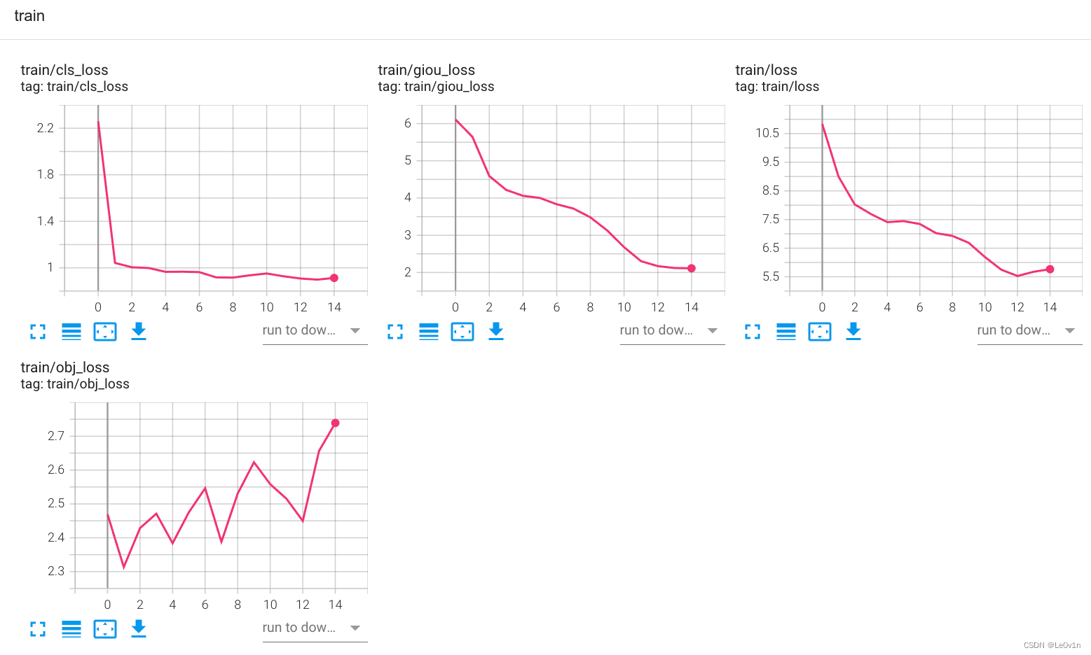
训练演示结果如下:
Test:   [1400/1456]  eta: 0:00:02.518983  model_time: 0.0323 (0.0367)  evaluator_time: 0.0080 (0.0065)  time: 0.0386  data: 0.0001  max mem: 759
Test:   [1455/1456]  eta: 0:00:00.044730  model_time: 0.0220 (0.0365)  evaluator_time: 0.0038 (0.0064)  time: 0.0371  data: 0.0001  max mem: 759
Test:  Total time: 0:01:05 (0.0448 s / it)
Averaged stats: model_time: 0.0220 (0.0365)  evaluator_time: 0.0038 (0.0064)
Accumulating evaluation results...
DONE (t=1.48s).
IoU metric: bbox
 Average Precision  (AP) @[ IoU=0.50:0.95 | area=   all | maxDets=100 ] = 0.571
 Average Precision  (AP) @[ IoU=0.50      | area=   all | maxDets=100 ] = 0.796
 Average Precision  (AP) @[ IoU=0.75      | area=   all | maxDets=100 ] = 0.635
 Average Precision  (AP) @[ IoU=0.50:0.95 | area= small | maxDets=100 ] = 0.199
 Average Precision  (AP) @[ IoU=0.50:0.95 | area=medium | maxDets=100 ] = 0.461
 Average Precision  (AP) @[ IoU=0.50:0.95 | area= large | maxDets=100 ] = 0.655
 Average Recall     (AR) @[ IoU=0.50:0.95 | area=   all | maxDets=  1 ] = 0.460
 Average Recall     (AR) @[ IoU=0.50:0.95 | area=   all | maxDets= 10 ] = 0.676
 Average Recall     (AR) @[ IoU=0.50:0.95 | area=   all | maxDets=100 ] = 0.692
 Average Recall     (AR) @[ IoU=0.50:0.95 | area= small | maxDets=100 ] = 0.338
 Average Recall     (AR) @[ IoU=0.50:0.95 | area=medium | maxDets=100 ] = 0.599
 Average Recall     (AR) @[ IoU=0.50:0.95 | area= large | maxDets=100 ] = 0.756
2.2. 预测脚本
import os
import json
import time

import torch
import cv2
import numpy as np
import matplotlib
matplotlib.use("TkAgg")
from matplotlib import pyplot as plt
from PIL import Image

from build_utils import img_utils, torch_utils, utils
from models import Darknet
from draw_box_utils import draw_objs


def main():
    img_size = 512  # 必须是32的整数倍 [416, 512, 608]
    cfg = "cfg/my_yolov3.cfg"  # 改成生成的.cfg文件
    weights = "weights/yolov3spp-14.pt"  # 改成自己训练好的权重文件
    json_path = "./data/pascal_voc_classes.json"  # json标签文件
    img_path = "test.png"
    assert os.path.exists(cfg), "cfg file {} dose not exist.".format(cfg)
    assert os.path.exists(weights), "weights file {} dose not exist.".format(weights)
    assert os.path.exists(json_path), "json file {} dose not exist.".format(json_path)
    assert os.path.exists(img_path), "image file {} dose not exist.".format(img_path)

    with open(json_path, 'r') as f:
        class_dict = json.load(f)

    category_index = {

    str(v): str(k) for k, v in class_dict.items()}

    input_size = (img_size, img_size)

    device = torch.device("cuda:0" if torch.cuda.is_available() else "cpu")

    model = Darknet(cfg, img_size)
    model.load_state_dict(torch.load(weights, map_location='cpu')["model"])
    model.to(device)

    model.eval()
    with torch.no_grad():  # 禁止梯度跟踪
        # init
        """
            在初始化时首先生成一个空的文件,传入网络进行正向传播
            原因:第一次调用网络是比较慢的(网络需要进行各种初始化)
        """
        img = torch.zeros((1, 3, img_size, img_size), device=device)
        model(img)

        img_o = cv2.imread(img_path)  # BGR(OpenCV读取图片的格式是BGR,后面需对去进行转换)
        assert img_o is not None, "Image Not Found " + img_path

        """
            对图片进行调整
                auto=True表示将图片的最大边长调整为512,短边使用(0,0,0)像素进行填充,保证其短边也是32的整数倍
                整张图片并不是512×512 —— 可以减少网络的运算量
        """
        img = img_utils.letterbox(img_o, new_shape=input_size, auto=True, color=(0, 0, 0))[0]

        # Convert
        img = img[:, :, ::-1].transpose(2, 0, 1)  # BGR to RGB, to 3x416x416
        img = np.ascontiguousarray(img)  # 判断图片在内存中是否为连续,如果不是则对其进行调整(使其在内存中连续)

        img = torch.from_numpy(img).to(device).float()
        img /= 255.0  # scale (0, 255) to (0, 1) —— 只将其调整为[0, 1],并没有进行标准化
        img = img.unsqueeze(0)  # add batch dimension

        t1 = torch_utils.time_synchronized()
        pred = model(img)[0]  # only get inference result
        t2 = torch_utils.time_synchronized()
        print(t2 - t1)

        pred = utils.non_max_suppression(pred, conf_thres=0.1, iou_thres=0.6, multi_label=True)[0]
        t3 = time.time()
        print(t3 - t2)

        if pred is None:
            print("No target detected.")
            exit(0)

        # process detections
        """
            将得到的目标边界框映射到原图像的尺度上
        """
        pred[:, :4] = utils.scale_coords(img.shape[2:], pred[:, :4], img_o.shape).round()
        print(pred.shape)

        bboxes = pred[:, :4].detach().cpu().numpy()
        scores = pred[:, 4].detach().cpu().numpy()
        classes = pred[:, 5].detach().cpu().numpy().astype(np.int) + 1

        pil_img = Image.fromarray(img_o[:, :, ::-1])
        plot_img = draw_objs(pil_img,
                             bboxes,
                             classes,
                             scores,
                             category_index=category_index,
                             box_thresh=0.2,
                             line_thickness=3,
                             font='arial.ttf',
                             font_size=20)
        plt.imshow(plot_img)
        plt.show()
        # 保存预测的图片结果
        plot_img.save("test_result.jpg")


if __name__ == "__main__":
    main()

3. 配置文件 —— cfg/yolov3-spp.cfg
这是YOLO v3-SPP的配置文件,这个文件告诉项目应该如何搭建网络。里面有以下几个块:
[convolutional][shortcut][maxpool][route][upsample][yolo]
3.1 [convolutional]
[convolutional]	—— 卷积层
batch_normalize=1	—— BN层,1表示使用BN层,0表示不使用BN层(如果使用BN层,建议卷积层的bias设置为False)。
filters=32	—— 卷积层中卷积核的个数(输出特征图的channel)
size=3	—— 卷积核的尺寸
stride=1	—— 卷积核的步长
pad=1	—— 是否启用padding,如果为1则padding = kernel_size // 2,如果为0,则padding = 0
activation=leaky —— 使用什么激活函数
3.2 [shortcut]
[shortcut]	—— 捷径分支
from=-3	—— 与前面哪一层的输出进行融合(两个shape完全一样的特征图相加的操作)
activation=linear —— 线性激活(对输入不做任何处理 — y=x)

3.3 [maxpool]
在YOLO v3原版中是没有MaxPooling层的。在YOLO v3-SPP中,MaxPooling只出现在SPP结构中。
[maxpool] —— MaxPooling层
stride=1 —— 池化核步长
size=5  ——池化核尺寸
MaxPooling的padding = (kernel_size - 1) // 2
这说明如果MaxPooling的stride=1,不进行下采样;stride=2,进行两倍下采样
3.4 [route]
route 英
[ruːt]美[ruːt]
n. 路线; 路途; (公共汽车和列车等的)常规路线,固定线路; 途径; 渠道; (用于美国干线公路号码前);
vt. 按某路线发送;
这个层结构有两种形式,当route有一个值和多个值,对应的操作是不一样的。
3.4.1 [route]取一个值
[route]
layers=-2
当layer只有一个值的时候,代表指向某一层的输出
3.4.2 [route]取多个值
[route]
layers=-1,-3,-5,-6
当layer有多个值的时候,代表将多个输出进行拼接(在通道维度进行拼接 —— shape相同,channel相加)
3.5 搭建SPP
为了更加容易理解[route],我们看一下SPP是怎么在yolov3-spp.cfg文件中搭建的。
SPP结构如下图所示:

configuration对应的内容如下:
[convolutional] —— SPP前的一个卷积层
batch_normalize=1
filters=512
size=1
stride=1
pad=1
activation=leaky

### SPP ###
[maxpool]
stride=1
size=5

[route]
layers=-2

[maxpool]
stride=1
size=9

[route]
layers=-4

[maxpool]
stride=1
size=13

[route]
layers=-1,-3,-5,-6

### End SPP ###
通过SPP图我们可以看到,特征图在进入SPP之前是经过一个Conv层的 --> MaxPooling层(5×5/1) --> route层(layer=-2,layer只有一个值,所以是指向-2层的) --> 将输出指向Conv层 --> MaxPooling层(9×9/1) --> route层(layer=-4,layer只有一个值,所以是指向-4层的) --> 将输出指向Conv层 --> MaxPooling层(13×13/1)–> route(layer=-1,-3,-5,-6,layer有多个数值表示将多层的输出进行维度拼接 —— shape相同,channel相加)

对于layer来说,当前层为0
3.6 [upsample]
[upsample] —— 上采样层
stride=2 —— 上采样倍率
在原版YOLO v3中是没有上采样层的,在YOLO v3-SPP中上采样层出现在两个地方:
- SPP第一个predict layer到第二个predict layer之间
- SPP第二个predict layer到第三个predict layer之间

这里上采样层的作用是:将特征图的 H , W H, W H,W放大到原来的2倍。
3.7 [yolo]
[yolo] —— yolo层(这里的yolo层并不是用于预测的predictor,yolo层是接在每个predictor之后的结构。它存在的意义是对predictor的结果进行处理以及生成一系列的anchors)
mask = 6,7,8  —— 使用哪些anchor priors(对应的是索引,从0开始)
anchors = 10,13,  16,30,  33,23,  30,61,  62,45,  59,119,  116,90,  156,198,  373,326 —— 对应YOLO v3采用的anchor priors(两两为一组,分别代码anchor priors的宽度W和高度H)
classes=80 —— 目标类别个数(这里的80是COCO数据集的类别个数)
num=9 —— 没有使用到的参数
jitter=.3 —— 没有使用到的参数
ignore_thresh = .7 —— 没有使用到的参数
truth_thresh = 1 —— 没有使用到的参数
random=1 —— 没有使用到的参数

注意:
- 这里的yolo层并不是用于预测的predictor,yolo层是接在每个predictor之后的结构。
它存在的意义是对predictor的结果进行处理以及生成一系列的anchors - anchors = 10,13, 16,30, 33,23, 30,61, 62,45, 59,119, 116,90, 156,198, 373,326 —— 对应YOLO v3采用的anchor priors(两两为一组,分别代表anchor priors的宽度W和高度H)
- 10,13, 16,30, 33,23:小目标的anchor priors(对应的predictor为52×52)——mask对应的索引为 0,1,2
- 30,61, 62,45, 59,119:中目标的anchor priors(对应的predictor为26×26)——mask对应的索引为 4,5,6
- 116,90, 156,198, 373,326:大目标的anchor priors(对应的predictor为13×13)——mask对应的索引为 7,8,9
4. yolov3-spp.cfg解析
import os
import numpy as np


def parse_model_cfg(path: str):  # path为yolov3-spp.cfg的路径
    # 检查文件是否存在
    if not path.endswith(".cfg") or not os.path.exists(path):
        raise FileNotFoundError("the cfg file not exist...")

    # 读取文件信息
    with open(path, "r") as f:
        lines = f.read().split("\n")

    # 去除空行和注释行
    lines = [x for x in lines if x and not x.startswith("#")]  # if x:表示当前行不为空
    # 去除每行开头和结尾的空格符
    lines = [x.strip() for x in lines]

    mdefs = []  # module definitions
    for line in lines:
        if line.startswith("["):  # this marks the start of a new block
            mdefs.append({

    })
            mdefs[-1]["type"] = line[1:-1].strip()  # 记录module类型 -> {type: 层结构的名称}
            # 如果是卷积模块,设置默认不使用BN(普通卷积层后面会重写成1,最后的预测层conv保持为0)
            if mdefs[-1]["type"] == "convolutional":
                mdefs[-1]["batch_normalize"] = 0
        else:  # 如果不是以[开头 -> 说明是一系列参数
            key, val = line.split("=")  # 通过=分割
            key = key.strip()  # 变量名
            val = val.strip()  # 内容

            """
                Note:读取进来的都会自动转换为str类似,所以如果是数值我们需要再转换为对应的数据类型(int/float)
            """
            if key == "anchors":  # yolo层中的anchors
                # anchors = 10,13,  16,30,  33,23,  30,61,  62,45,  59,119,  116,90,  156,198,  373,326
                val = val.replace(" ", "")  # 将空格去除
                mdefs[-1][key] = np.array([float(x) for x in val.split(",")]).reshape((-1, 2))  # np anchors
            elif (key in ["from", "layers", "mask"]) or (key == "size" and "," in val):
                mdefs[-1][key] = [int(x) for x in val.split(",")]
            else:
                # TODO: .isnumeric() actually fails to get the float case
                if val.isnumeric():  # return int or float 如果是数值的情况
                    """
                        判断其是int还是float
                            >>> val = 3
                            >>> int(val) if (int(val) - float(val)) == 0 else float(val)
                            3
                            >>> val = 3.5
                            >>> int(val) if (int(val) - float(val)) == 0 else float(val)
                            3.5
                    """
                    mdefs[-1][key] = int(val) if (int(val) - float(val)) == 0 else float(val)
                else:
                    mdefs[-1][key] = val  # return string  是字符的情况

    # check all fields are supported
    supported = ['type', 'batch_normalize', 'filters', 'size', 'stride', 'pad', 'activation', 'layers', 'groups',
                 'from', 'mask', 'anchors', 'classes', 'num', 'jitter', 'ignore_thresh', 'truth_thresh', 'random',
                 'stride_x', 'stride_y', 'weights_type', 'weights_normalization', 'scale_x_y', 'beta_nms', 'nms_kind',
                 'iou_loss', 'iou_normalizer', 'cls_normalizer', 'iou_thresh', 'probability']

    # 遍历检查每个模型的配置
    for x in mdefs[1:]:  # 0对应net配置(这个我们是不会使用到的)
        # 遍历每个配置字典中的key值
        for k in x:
            if k not in supported:
                raise ValueError("Unsupported fields:{} in cfg".format(k))

    return mdefs


def parse_data_cfg(path):
    # Parses the data configuration file
    if not os.path.exists(path) and os.path.exists('data' + os.sep + path):  # add data/ prefix if omitted
        path = 'data' + os.sep + path

    with open(path, 'r') as f:
        lines = f.readlines()

    options = dict()
    for line in lines:
        line = line.strip()
        if line == '' or line.startswith('#'):
            continue
        key, val = line.split('=')
        options[key.strip()] = val.strip()

    return options
我们可以开一下解析得到的list:
[{'type': 'net', 'batch': 64, 'subdivisions': 16, 'width': 608, 'height': 608, 'channels': 3, 'momentum': '0.9', 'decay': '0.0005', 'angle': 0, 'saturation': '1.5', 'exposure': '1.5', 'hue': '.1', 'learning_rate': '0.001', 'burn_in': 1000, 'max_batches': 500200, 'policy': 'steps', 'steps': '400000,450000', 'scales': '.1,.1'}, {'type': 'convolutional', 'batch_normalize': 1, 'filters': 32, 'size': 3, 'stride': 1, 'pad': 1, 'activation': 'leaky'}, {'type': 'convolutional', 'batch_normalize': 1, 'filters': 64, 'size': 3, 'stride': 2, 'pad': 1, 'activation': 'leaky'}, {'type': 'convolutional', 'batch_normalize': 1, 'filters': 32, 'size': 1, 'stride': 1, 'pad': 1, 'activation': 'leaky'}, {'type': 'convolutional', 'batch_normalize': 1, 'filters': 64, 'size': 3, 'stride': 1, 'pad': 1, 'activation': 'leaky'}, {'type': 'shortcut', 'from': [-3], 'activation': 'linear'}, {'type': 'convolutional', 'batch_normalize': 1, 'filters': 128, 'size': 3, 'stride': 2, 'pad': 1, 'activation': 'leaky'}, {'type': 'convolutional', 'batch_normalize': 1, 'filters': 64, 'size': 1, 'stride': 1, 'pad': 1, 'activation': 'leaky'}, {'type': 'convolutional', 'batch_normalize': 1, 'filters': 128, 'size': 3, 'stride': 1, 'pad': 1, 'activation': 'leaky'}, {'type': 'shortcut', 'from': [-3], 'activation': 'linear'}, {'type': 'convolutional', 'batch_normalize': 1, 'filters': 64, 'size': 1, 'stride': 1, 'pad': 1, 'activation': 'leaky'}, {'type': 'convolutional', 'batch_normalize': 1, 'filters': 128, 'size': 3, 'stride': 1, 'pad': 1, 'activation': 'leaky'}, {'type': 'shortcut', 'from': [-3], 'activation': 'linear'}, {'type': 'convolutional', 'batch_normalize': 1, 'filters': 256, 'size': 3, 'stride': 2, 'pad': 1, 'activation': 'leaky'}, {'type': 'convolutional', 'batch_normalize': 1, 'filters': 128, 'size': 1, 'stride': 1, 'pad': 1, 'activation': 'leaky'}, {'type': 'convolutional', 'batch_normalize': 1, 'filters': 256, 'size': 3, 'stride': 1, 'pad': 1, 'activation': 'leaky'}, {'type': 'shortcut', 'from': [-3], 'activation': 'linear'}, {'type': 'convolutional', 'batch_normalize': 1, 'filters': 128, 'size': 1, 'stride': 1, 'pad': 1, 'activation': 'leaky'}, {'type': 'convolutional', 'batch_normalize': 1, 'filters': 256, 'size': 3, 'stride': 1, 'pad': 1, 'activation': 'leaky'}, {'type': 'shortcut', 'from': [-3], 'activation': 'linear'}, {'type': 'convolutional', 'batch_normalize': 1, 'filters': 128, 'size': 1, 'stride': 1, 'pad': 1, 'activation': 'leaky'}, {'type': 'convolutional', 'batch_normalize': 1, 'filters': 256, 'size': 3, 'stride': 1, 'pad': 1, 'activation': 'leaky'}, {'type': 'shortcut', 'from': [-3], 'activation': 'linear'}, {'type': 'convolutional', 'batch_normalize': 1, 'filters': 128, 'size': 1, 'stride': 1, 'pad': 1, 'activation': 'leaky'}, {'type': 'convolutional', 'batch_normalize': 1, 'filters': 256, 'size': 3, 'stride': 1, 'pad': 1, 'activation': 'leaky'}, {'type': 'shortcut', 'from': [-3], 'activation': 'linear'}, {'type': 'convolutional', 'batch_normalize': 1, 'filters': 128, 'size': 1, 'stride': 1, 'pad': 1, 'activation': 'leaky'}, {'type': 'convolutional', 'batch_normalize': 1, 'filters': 256, 'size': 3, 'stride': 1, 'pad': 1, 'activation': 'leaky'}, {'type': 'shortcut', 'from': [-3], 'activation': 'linear'}, {'type': 'convolutional', 'batch_normalize': 1, 'filters': 128, 'size': 1, 'stride': 1, 'pad': 1, 'activation': 'leaky'}, {'type': 'convolutional', 'batch_normalize': 1, 'filters': 256, 'size': 3, 'stride': 1, 'pad': 1, 'activation': 'leaky'}, {'type': 'shortcut', 'from': [-3], 'activation': 'linear'}, {'type': 'convolutional', 'batch_normalize': 1, 'filters': 128, 'size': 1, 'stride': 1, 'pad': 1, 'activation': 'leaky'}, {'type': 'convolutional', 'batch_normalize': 1, 'filters': 256, 'size': 3, 'stride': 1, 'pad': 1, 'activation': 'leaky'}, {'type': 'shortcut', 'from': [-3], 'activation': 'linear'}, {'type': 'convolutional', 'batch_normalize': 1, 'filters': 128, 'size': 1, 'stride': 1, 'pad': 1, 'activation': 'leaky'}, {'type': 'convolutional', 'batch_normalize': 1, 'filters': 256, 'size': 3, 'stride': 1, 'pad': 1, 'activation': 'leaky'}, {'type': 'shortcut', 'from': [-3], 'activation': 'linear'}, {'type': 'convolutional', 'batch_normalize': 1, 'filters': 512, 'size': 3, 'stride': 2, 'pad': 1, 'activation': 'leaky'}, {'type': 'convolutional', 'batch_normalize': 1, 'filters': 256, 'size': 1, 'stride': 1, 'pad': 1, 'activation': 'leaky'}, {'type': 'convolutional', 'batch_normalize': 1, 'filters': 512, 'size': 3, 'stride': 1, 'pad': 1, 'activation': 'leaky'}, {'type': 'shortcut', 'from': [-3], 'activation': 'linear'}, {'type': 'convolutional', 'batch_normalize': 1, 'filters': 256, 'size': 1, 'stride': 1, 'pad': 1, 'activation': 'leaky'}, {'type': 'convolutional', 'batch_normalize': 1, 'filters': 512, 'size': 3, 'stride': 1, 'pad': 1, 'activation': 'leaky'}, {'type': 'shortcut', 'from': [-3], 'activation': 'linear'}, {'type': 'convolutional', 'batch_normalize': 1, 'filters': 256, 'size': 1, 'stride': 1, 'pad': 1, 'activation': 'leaky'}, {'type': 'convolutional', 'batch_normalize': 1, 'filters': 512, 'size': 3, 'stride': 1, 'pad': 1, 'activation': 'leaky'}, {'type': 'shortcut', 'from': [-3], 'activation': 'linear'}, {'type': 'convolutional', 'batch_normalize': 1, 'filters': 256, 'size': 1, 'stride': 1, 'pad': 1, 'activation': 'leaky'}, {'type': 'convolutional', 'batch_normalize': 1, 'filters': 512, 'size': 3, 'stride': 1, 'pad': 1, 'activation': 'leaky'}, {'type': 'shortcut', 'from': [-3], 'activation': 'linear'}, {'type': 'convolutional', 'batch_normalize': 1, 'filters': 256, 'size': 1, 'stride': 1, 'pad': 1, 'activation': 'leaky'}, {'type': 'convolutional', 'batch_normalize': 1, 'filters': 512, 'size': 3, 'stride': 1, 'pad': 1, 'activation': 'leaky'}, {'type': 'shortcut', 'from': [-3], 'activation': 'linear'}, {'type': 'convolutional', 'batch_normalize': 1, 'filters': 256, 'size': 1, 'stride': 1, 'pad': 1, 'activation': 'leaky'}, {'type': 'convolutional', 'batch_normalize': 1, 'filters': 512, 'size': 3, 'stride': 1, 'pad': 1, 'activation': 'leaky'}, {'type': 'shortcut', 'from': [-3], 'activation': 'linear'}, {'type': 'convolutional', 'batch_normalize': 1, 'filters': 256, 'size': 1, 'stride': 1, 'pad': 1, 'activation': 'leaky'}, {'type': 'convolutional', 'batch_normalize': 1, 'filters': 512, 'size': 3, 'stride': 1, 'pad': 1, 'activation': 'leaky'}, {'type': 'shortcut', 'from': [-3], 'activation': 'linear'}, {'type': 'convolutional', 'batch_normalize': 1, 'filters': 256, 'size': 1, 'stride': 1, 'pad': 1, 'activation': 'leaky'}, {'type': 'convolutional', 'batch_normalize': 1, 'filters': 512, 'size': 3, 'stride': 1, 'pad': 1, 'activation': 'leaky'}, {'type': 'shortcut', 'from': [-3], 'activation': 'linear'}, {'type': 'convolutional', 'batch_normalize': 1, 'filters': 1024, 'size': 3, 'stride': 2, 'pad': 1, 'activation': 'leaky'}, {'type': 'convolutional', 'batch_normalize': 1, 'filters': 512, 'size': 1, 'stride': 1, 'pad': 1, 'activation': 'leaky'}, {'type': 'convolutional', 'batch_normalize': 1, 'filters': 1024, 'size': 3, 'stride': 1, 'pad': 1, 'activation': 'leaky'}, {'type': 'shortcut', 'from': [-3], 'activation': 'linear'}, {'type': 'convolutional', 'batch_normalize': 1, 'filters': 512, 'size': 1, 'stride': 1, 'pad': 1, 'activation': 'leaky'}, {'type': 'convolutional', 'batch_normalize': 1, 'filters': 1024, 'size': 3, 'stride': 1, 'pad': 1, 'activation': 'leaky'}, {'type': 'shortcut', 'from': [-3], 'activation': 'linear'}, {'type': 'convolutional', 'batch_normalize': 1, 'filters': 512, 'size': 1, 'stride': 1, 'pad': 1, 'activation': 'leaky'}, {'type': 'convolutional', 'batch_normalize': 1, 'filters': 1024, 'size': 3, 'stride': 1, 'pad': 1, 'activation': 'leaky'}, {'type': 'shortcut', 'from': [-3], 'activation': 'linear'}, {'type': 'convolutional', 'batch_normalize': 1, 'filters': 512, 'size': 1, 'stride': 1, 'pad': 1, 'activation': 'leaky'}, {'type': 'convolutional', 'batch_normalize': 1, 'filters': 1024, 'size': 3, 'stride': 1, 'pad': 1, 'activation': 'leaky'}, {'type': 'shortcut', 'from': [-3], 'activation': 'linear'}, {'type': 'convolutional', 'batch_normalize': 1, 'filters': 512, 'size': 1, 'stride': 1, 'pad': 1, 'activation': 'leaky'}, {'type': 'convolutional', 'batch_normalize': 1, 'size': 3, 'stride': 1, 'pad': 1, 'filters': 1024, 'activation': 'leaky'}, {'type': 'convolutional', 'batch_normalize': 1, 'filters': 512, 'size': 1, 'stride': 1, 'pad': 1, 'activation': 'leaky'}, {'type': 'maxpool', 'stride': 1, 'size': 5}, {'type': 'route', 'layers': [-2]}, {'type': 'maxpool', 'stride': 1, 'size': 9}, {'type': 'route', 'layers': [-4]}, {'type': 'maxpool', 'stride': 1, 'size': 13}, {'type': 'route', 'layers': [-1, -3, -5, -6]}, {'type': 'convolutional', 'batch_normalize': 1, 'filters': 512, 'size': 1, 'stride': 1, 'pad': 1, 'activation': 'leaky'}, {'type': 'convolutional', 'batch_normalize': 1, 'size': 3, 'stride': 1, 'pad': 1, 'filters': 1024, 'activation': 'leaky'}, {'type': 'convolutional', 'batch_normalize': 1, 'filters': 512, 'size': 1, 'stride': 1, 'pad': 1, 'activation': 'leaky'}, {'type': 'convolutional', 'batch_normalize': 1, 'size': 3, 'stride': 1, 'pad': 1, 'filters': 1024, 'activation': 'leaky'}, {'type': 'convolutional', 'batch_normalize': 0, 'size': 1, 'stride': 1, 'pad': 1, 'filters': 75, 'activation': 'linear'}, {'type': 'yolo', 'mask': [6, 7, 8], 'anchors': array([[         10,          13],
       [         16,          30],
       [         33,          23],
       [         30,          61],
       [         62,          45],
       [         59,         119],
       [        116,          90],
       [        156,         198],
       [        373,         326]]), 'classes': 20, 'num': 9, 'jitter': '.3', 'ignore_thresh': '.7', 'truth_thresh': 1, 'random': 1}, {'type': 'route', 'layers': [-4]}, {'type': 'convolutional', 'batch_normalize': 1, 'filters': 256, 'size': 1, 'stride': 1, 'pad': 1, 'activation': 'leaky'}, {'type': 'upsample', 'stride': 2}, {'type': 'route', 'layers': [-1, 61]}, {'type': 'convolutional', 'batch_normalize': 1, 'filters': 256, 'size': 1, 'stride': 1, 'pad': 1, 'activation': 'leaky'}, {'type': 'convolutional', 'batch_normalize': 1, 'size': 3, 'stride': 1, 'pad': 1, 'filters': 512, 'activation': 'leaky'}, {'type': 'convolutional', 'batch_normalize': 1, 'filters': 256, 'size': 1, 'stride': 1, 'pad': 1, 'activation': 'leaky'}, {'type': 'convolutional', 'batch_normalize': 1, 'size': 3, 'stride': 1, 'pad': 1, 'filters': 512, 'activation': 'leaky'}, {'type': 'convolutional', 'batch_normalize': 1, 'filters': 256, 'size': 1, 'stride': 1, 'pad': 1, 'activation': 'leaky'}, {'type': 'convolutional', 'batch_normalize': 1, 'size': 3, 'stride': 1, 'pad': 1, 'filters': 512, 'activation': 'leaky'}, {'type': 'convolutional', 'batch_normalize': 0, 'size': 1, 'stride': 1, 'pad': 1, 'filters': 75, 'activation': 'linear'}, {'type': 'yolo', 'mask': [3, 4, 5], 'anchors': array([[         10,          13],
       [         16,          30],
       [         33,          23],
       [         30,          61],
       [         62,          45],
       [         59,         119],
       [        116,          90],
       [        156,         198],
       [        373,         326]]), 'classes': 20, 'num': 9, 'jitter': '.3', 'ignore_thresh': '.7', 'truth_thresh': 1, 'random': 1}, {'type': 'route', 'layers': [-4]}, {'type': 'convolutional', 'batch_normalize': 1, 'filters': 128, 'size': 1, 'stride': 1, 'pad': 1, 'activation': 'leaky'}, {'type': 'upsample', 'stride': 2}, {'type': 'route', 'layers': [-1, 36]}, {'type': 'convolutional', 'batch_normalize': 1, 'filters': 128, 'size': 1, 'stride': 1, 'pad': 1, 'activation': 'leaky'}, {'type': 'convolutional', 'batch_normalize': 1, 'size': 3, 'stride': 1, 'pad': 1, 'filters': 256, 'activation': 'leaky'}, {'type': 'convolutional', 'batch_normalize': 1, 'filters': 128, 'size': 1, 'stride': 1, 'pad': 1, 'activation': 'leaky'}, {'type': 'convolutional', 'batch_normalize': 1, 'size': 3, 'stride': 1, 'pad': 1, 'filters': 256, 'activation': 'leaky'}, {'type': 'convolutional', 'batch_normalize': 1, 'filters': 128, 'size': 1, 'stride': 1, 'pad': 1, 'activation': 'leaky'}, {'type': 'convolutional', 'batch_normalize': 1, 'size': 3, 'stride': 1, 'pad': 1, 'filters': 256, 'activation': 'leaky'}, {'type': 'convolutional', 'batch_normalize': 0, 'size': 1, 'stride': 1, 'pad': 1, 'filters': 75, 'activation': 'linear'}, {'type': 'yolo', 'mask': [0, 1, 2], 'anchors': array([[         10,          13],
       [         16,          30],
       [         33,          23],
       [         30,          61],
       [         62,          45],
       [         59,         119],
       [        116,          90],
       [        156,         198],
       [        373,         326]]), 'classes': 20, 'num': 9, 'jitter': '.3', 'ignore_thresh': '.7', 'truth_thresh': 1, 'random': 1}]
Backend TkAgg is interactive backend. Turning interactive mode on.
5. Darknet网络定义
from build_utils.layers import *
from build_utils.parse_config import *
import build_utils.torch_utils as torch_utils
ONNX_EXPORT = False
def create_modules(modules_defs: list, img_size):
"""
Constructs module list of layer blocks from module configuration in module_defs
:param modules_defs: 通过.cfg文件解析得到的每个层结构的列表
:param img_size:
:return:
1. module_list: 网络中各个层
2. routs_binary: mask(被后面层调用的层结构位置为True) —— 记录哪一层的输入要被保存
"""
img_size = [img_size] * 2 if isinstance(img_size, int) else img_size
# 删除解析cfg列表中的第一个配置(对应[net]的配置)
modules_defs.pop(0) # cfg training hyperparams (unused)
"""
output_filters: 记录每一个模块的输出channel
在“遍历搭建每个层结构”中,每次遍历都会追加输出的通道数
"""
output_filters = [3] # input channels
module_list = nn.ModuleList()
"""
routs: 统计哪些特征层的输出会被后续的层使用到(可能是特征融合,也可能是拼接)
[1, 5, 8, 12, 15, 18, 21, 24, 27, 30, 33, 37, 40, 43, 46, 49, 52, 55, 58, 62, 65, 68, 71]
也就是说,routs中记录网络层的索引
"""
routs = [] # list of layers which rout to deeper layers
yolo_index = -1
# 遍历搭建每个层结构
for i, mdef in enumerate(modules_defs):
modules = nn.Sequential()
if mdef["type"] == "convolutional":
bn = mdef["batch_normalize"] # 1 or 0 / use or not
filters = mdef["filters"]
k = mdef["size"] # kernel size
# YOLO v3-SPP中每一个Convolutional都有stride参数,所以可以不用管else (mdef['stride_y'], mdef["stride_x"]这个参数
stride = mdef["stride"] if "stride" in mdef else (mdef['stride_y'], mdef["stride_x"])
if isinstance(k, int):
modules.add_module("Conv2d", nn.Conv2d(in_channels=output_filters[-1],
out_channels=filters,
kernel_size=k,
stride=stride,
padding=k // 2 if mdef["pad"] else 0,
bias=not bn))
else:
raise TypeError("conv2d filter size must be int type.")
if bn:
modules.add_module("BatchNorm2d", nn.BatchNorm2d(filters))
else:
# 如果该卷积操作没有bn层,意味着该层为yolo的predictor -> 记录predictor的索引
routs.append(i) # detection output (goes into yolo layer)
if mdef["activation"] == "leaky":
modules.add_module("activation", nn.LeakyReLU(0.1, inplace=True))
else:
pass
elif mdef["type"] == "BatchNorm2d":
pass
elif mdef["type"] == "maxpool": # 5×5、9×9、13×13
k = mdef["size"] # kernel size
stride = mdef["stride"]
modules = nn.MaxPool2d(kernel_size=k, stride=stride, padding=(k - 1) // 2)
elif mdef["type"] == "upsample":
if ONNX_EXPORT: # explicitly state size, avoid scale_factor
g = (yolo_index + 1) * 2 / 32 # gain
modules = nn.Upsample(size=tuple(int(x * g) for x in img_size))
else:
modules = nn.Upsample(scale_factor=mdef["stride"])
elif mdef["type"] == "route": # [-2], [-1,-3,-5,-6], [-1, 61]
layers = mdef["layers"]
"""
filters: 记录当前层输出特征图的channel
遍历layers这个列表,得到这个list中的每一个值l。
+ 如果l>0的话,则需要output_filters[l + 1]。这是因为在定义output_filfer时是这样定义的:
output_filter = [3],即创建了一个list且第0个元素的值为3(输入特征图通道数为3)。
>>> a = [3]
>>> a
[3]
因此output_filters[0]并不是第一个block的输出,而是输入图片的channel,这个channel是不算的
因此要让l+1得到第一个block的输出(l是从开始的) -> output_filter[l + 1]
+ 如果l<0的话,则可以直接写入l,因为对于output_filfer[l],l<0是倒着数的,顺序是不会出现问题的
(不太可能倒着数还出问题)
filters = sum([output_filters[l + 1 if l > 0 else l] for l in layers])
+ 当layers只有一个值的时候,得到的结果就是指向模块输出特征图的通道数 -> 一个数
+ 当layers为多个值时,就将layers中指向一系列层结构的输出特征图的通道数求和∑,得到最终concat后的channel -> 一个数
"""
filters = sum([output_filters[l + 1 if l > 0 else l] for l in layers])
"""
首先要明确一件事情:
filter: 保存模块输出特征图的channel
routs: 模块的索引(记录的就是就是模型从头到尾每一层的idx)
list.extend() 函数用于在列表末尾一次性追加另一个序列中的多个值(用新列表扩展原来的列表)
[i + l if l < 0 else l for l in layers]:
遍历layers中的每一个元素l:
+ 当l<0时,说明要记录模块的索引是相对索引(即是根据当前route模块往前推)索引为i+l(其中i为当前route模块的索引)
引入l=-1,即使用route层前面一个模块,所以模块的idx应该为当前route的索引值-1,即i+l
+ 当l>0,说明要记录模块的索引是绝对索引(即从网络整体来看的),所以直接记录为l即可
"""
routs.extend([i + l if l < 0 else l for l in layers])
modules = FeatureConcat(layers=layers)
elif mdef["type"] == "shortcut":
layers = mdef["from"] # from表示要与前面哪一层的输出进行融合,因为是针对残差结构,所以一般都是=-3的
filters = output_filters[-1] # -1就是取上一个模块的输出
"""
因为shortcut使用到了之前的输出,所以需要记录一下到底是使用哪一个层的输出
(i为当前层的索引,layers[0]是负数,表示前面第几层)
"""
# routs.extend([i + l if l < 0 else l for l in layers])
routs.append(i + layers[0])
"""
使用WeightedFeatureFusion这个类,将两个特征图进行特征融合(shape完全相同,直接加)
layers: 前面第几层
weights: 这个参数我们是没有使用到的,所以不用管它
"""
modules = WeightedFeatureFusion(layers=layers, weight="weights_type" in mdef)
elif mdef["type"] == "yolo":
"""
yolo_index初始化为-1
因为在YOLO v3-SPP中只有3个yolo层,
所以在yolo_index += 1后,
yolo_index属于[0, 1, 2]
"""
yolo_index += 1 # 记录是第几个yolo_layer [0, 1, 2]
stride = [32, 16, 8] # 预测特征层对应原图的缩放比例 -> [16×16, 32×32, 64×64]
"""
[yolo]
mask = 0,1,2 —— 所使用anchor priors的idx
anchors = 10,13, 16,30, 33,23, 30,61, 62,45, 59,119, 116,90, 156,198, 373,326
classes=80 —— 类别
"""
modules = YOLOLayer(anchors=mdef["anchors"][mdef["mask"]], # anchor list
nc=mdef["classes"], # number of classes
img_size=img_size, # 这个参数只有在模型导出为onnx时使用
stride=stride[yolo_index]) # 对应predictor预测特征图相对输入的缩放比例(下采样倍率)
"""
对每个predictor的偏置进行初始化
"""
# Initialize preceding Conv2d() bias (https://arxiv.org/pdf/1708.02002.pdf section 3.3)
try:
j = -1 # -1表示[yolo]的上一层,也就是对应的predictor
# bias: shape(255,) 索引0对应Sequential中的Conv2d
# view: shape(3, 85)
"""
module_list[j]去取上一个模块
module_list[j][0]表示取Sequential中的Conv2d
module_list[j][0].bias表示取其bias
"""
b = module_list[j][0].bias.view(modules.na, -1)
b.data[:, 4] += -4.5 # obj
b.data[:, 5:] += math.log(0.6 / (modules.nc - 0.99)) # cls (sigmoid(p) = 1/nc)
module_list[j][0].bias = torch.nn.Parameter(b.view(-1), requires_grad=True)
except Exception as e:
print('WARNING: smart bias initialization failure.', e)
else:
print("Warning: Unrecognized Layer Type: " + mdef["type"])
# Register module list and number of output filters
# 将上面得到的每一个module添加到module_list当中
module_list.append(modules)
"""
将每一个module的输出通道数添加到output_filters当中
(只有[convolutional][shortcut][route]中才有filters这个参数)
因为只有这些层当中它的特征图channel会发生变化
[maxpool][upsample]是不会改变特征图channel的
"""
output_filters.append(filters)
"""
构建一个routs_binary
[False, Flase, ..., False],长度为modules_defs —— yolov3-spp.cfg有多少个模块就有多少个False
modules_defs: 通过.cfg文件解析得到的每个层结构的列表
>>> [False] * 3
[False, False, False]
"""
routs_binary = [False] * len(modules_defs) # mask
"""
遍历routs列表:
routs: 统计哪些特征层的输出会被后续的层使用到(可能是特征融合,也可能是拼接)
[1, 5, 8, 12, 15, 18, 21, 24, 27, 30, 33, 37, 40, 43, 46, 49, 52, 55, 58, 62, 65, 68, 71]
也就是说,routs中记录网络层的索引
"""
for i in routs:
routs_binary[i] = True # 将相应位置的值设置为True
"""
module_list: 网络中各个层
routs_binary: mask(被后面调用的层结构位置为True) —— 记录哪一层的输入要被保存
"""
return module_list, routs_binary
class YOLOLayer(nn.Module):
"""
对YOLO的predictor的输出进行处理
Args:
p: predictor预测得到的参数
Returns:
io: [BS, anchor priors数量*grid_H*grid_W] -> 只对predictor的输出做view和permute处理
数值没有经过任何处理的
p: [BS, anchor priors数量, grid_H, grid_W, (5+20)] -> 最终目标边界框参数(
里面的数值加上了cell的左上角坐标)
"""
def __init__(self, anchors, nc, img_size, stride):
super(YOLOLayer, self).__init__()
self.anchors = torch.Tensor(anchors) # 将传入的anchors(numpy)转换为tensor
self.stride = stride # layer stride 特征图上一步对应原图上的步距 [32, 16, 8]
self.na = len(anchors) # number of anchors (3) 每个grid cell中生成anchor的个数(YOLO v3和YOLO v3-SPP都是3种尺度的anchor priors)
self.nc = nc # number of classes (80) # COCO:80; VOC:20
self.no = nc + 5 # 每一个anchor需预测的参数个数 number of outputs (85: x, y, w, h, obj, cls1, ...)
# nx, ny所用预测特征图的宽度和高度(16×16, 32×32, 64×64); ng为grid cell的size -> 这里简单初始化为0
self.nx, self.ny, self.ng = 0, 0, (0, 0) # initialize number of x, y gridpoints
# 将anchors大小缩放到grid尺度
"""
因为传入anchor priors的大小都是针对原图的尺度
anchors = 10,13, 16,30, 33,23, 30,61, 62,45, 59,119, 116,90, 156,198, 373,326
为了将其映射到预测特征图上,因此需要进行下采样(32, 16, 8)
self.anchor_vec.shape: [3, 2]:3为anchor的3种不同尺度(也可以理解为3种不同尺度的anchor priors),
2为anchor的W和H
"""
self.anchor_vec = self.anchors / self.stride
# batch_size, na, grid_h, grid_w, wh,
# 值为1的维度对应的值不是固定值,后续操作可根据broadcast广播机制自动扩充
self.anchor_wh = self.anchor_vec.view(1, self.na, 1, 1, 2) # [3, 2] -> [1, 3, 1, 1, 2]
"""
[1, 3, 1, 1, 2]
① [1] batch size
② [3] 每个grid cell生成的anchor priors的个数
③ [1] grid cell的高度
④ [1] grid cell的宽度
⑤ [2] 每一个anchor的宽度和高度
因为self.na和⑤是固定不变的,而①③④是随着输入数据不同发生变化的,
现在将其设置为1,这样即便数值发生变化,也会根据广播机制进行自动扩充
"""
self.grid = None
if ONNX_EXPORT:
self.training = False
self.create_grids((img_size[1] // stride, img_size[0] // stride)) # number x, y grid points
def create_grids(self, ng=(13, 13), device="cpu"):
"""
更新grids信息并生成新的grids参数
:param ng: 特征图大小 ng=(nx, ny) -> ny: predictor对应特征图(grid)的H nx: predictor对应特征图(grid)的W
:param device:
:return: self.grid: [1, 1, H, W, 2] = [BS, anchor的个数,grid高度,grid宽度,grid每个cell左上角的坐标]
前面两个[1,1]会根据广播机制自动扩充
"""
self.nx, self.ny = ng
self.ng = torch.tensor(ng, dtype=torch.float)
"""
构建每个cell(预测特征图每个像素)处的anchor的xy偏移量(在feature map上的)
"""
if not self.training: # 训练模式不需要回归到最终预测boxes(只需要计算Loss即可,不需要回归anchors)
"""
y, x = torch.meshgrid(a, b)的功能是生成网格,可以用于生成坐标。
函数输入两个一维张量a,b,返回两个tensor -> y,x
y, x的行数均为a的元素个数
y, x的列数均为b的元素个数
y: 记录y轴坐标
x: 记录x轴坐标
一般都会通过torch.stack((x, y), dim=2)方法将x, y拼接在一起
举个例子:
y, x = torch.meshgrid([torch.arange(4), torch.arange(6)])
grid = torch.stack((x, y), dim=2)
print(f"grid.shape: {grid.shape}")
print(f"grid:\n {grid}")
==================== Result ==================
grid.shape: torch.Size([4, 6, 2])
grid:
tensor([[[0, 0], [1, 0], [2, 0], [3, 0], [4, 0], [5, 0]],
[[0, 1], [1, 1], [2, 1], [3, 1], [4, 1], [5, 1]],
[[0, 2], [1, 2], [2, 2], [3, 2], [4, 2], [5, 2]],
[[0, 3], [1, 3], [2, 3], [3, 3], [4, 3], [5, 3]]])
"""
yv, xv = torch.meshgrid([torch.arange(self.ny, device=device),
torch.arange(self.nx, device=device)])
# batch_size, na, grid_h, grid_w, wh
"""
通过torch.stack方法生成grid,再更改其形状
[H, W, 2]=[grid高度,grid宽度,grid每个cell左上角的坐标]
-> [1, 1, H, W, 2] = [BS, anchor的个数,grid高度,grid宽度,grid每个cell左上角的坐标]
前面两个[1,1]会根据广播机制自动扩充
self.grid: 是grid网格,其中[..., :2]为每一个坐标为grid cell的左上角坐标
"""
self.grid = torch.stack((xv, yv), 2).view((1, 1, self.ny, self.nx, 2)).float()
if self.anchor_vec.device != device:
self.anchor_vec = self.anchor_vec.to(device)
self.anchor_wh = self.anchor_wh.to(device)
def forward(self, p):
"""
对YOLO predictor的输出进行处理的前向传播
Args:
p: predictor预测得到的参数
Returns:
io: [BS, anchor priors数量*grid_H*grid_W] -> 只对predictor的输出做view和permute处理
数值没有经过任何处理的
p: [BS, anchor priors数量, grid_H, grid_W, (5+20)] -> 最终目标边界框参数(
里面的数值加上了cell的左上角坐标)
"""
if ONNX_EXPORT:
bs = 1 # batch size
else:
"""
bs: predictor生成参数的batch size
_: predictor生成参数(这里我们不使用)
ny: predictor对应特征图(grid)的H
nx: predictor对应特征图的(grid)W
------------------------------------
这么理解:
+ grid就是predictor对应的特征图
+ cell就是grid(预测特征图)上的每一个像素
"""
bs, _, ny, nx = p.shape # batch_size, predict_param(255), grid(13), grid(13)
"""
判断self.nx和self.ny是否等于当前predictor的预测特征图的高度和宽度:
不相等:grid cell发生变化 -> 需重新生成grid cell参数
或者如果self.grid is None(第一次正向传播)-> 也需要生成grid cell参数
"""
if (self.nx, self.ny) != (nx, ny) or self.grid is None: # fix no grid bug
self.create_grids((nx, ny), p.device)
# view: (batch_size, 255, 13, 13) -> (batch_size, 3, 85, 13, 13)
# permute: (batch_size, 3, 85, 13, 13) -> (batch_size, 3, 13, 13, 85)
# [bs, anchor, grid, grid, xywh + obj + classes]
"""
p: predictor预测得到的特征矩阵
shape: [4, 75, 19, 19] = [BS, (5+20)*3, grid_H, grid_W]
① view: [BS, (5+20)*3, grid, grid] -> [BS, anchor priors数量, (5+20), grid_H, grid_W]=[BS, 3, 25, grid_H, grid_W]
② permute: [BS, anchor priors数量, (5+20), grid_H, grid_W] -> [BS, anchor priors数量, grid_H, grid_W, (5+20)]
③ contiguous: 使该tensor在内存中连续(通过permute方法改变原有tensor的排列顺序,在原有内存中不再连续了)
"""
p = p.view(bs, self.na, self.no, self.ny, self.nx).permute(0, 1, 3, 4, 2).contiguous() # prediction
if self.training:
return p
elif ONNX_EXPORT:
# Avoid broadcasting for ANE operations
m = self.na * self.nx * self.ny # 3*
ng = 1. / self.ng.repeat(m, 1)
grid = self.grid.repeat(1, self.na, 1, 1, 1).view(m, 2)
anchor_wh = self.anchor_wh.repeat(1, 1, self.nx, self.ny, 1).view(m, 2) * ng
p = p.view(m, self.no)
# xy = torch.sigmoid(p[:, 0:2]) + grid # x, y
# wh = torch.exp(p[:, 2:4]) * anchor_wh # width, height
# p_cls = torch.sigmoid(p[:, 4:5]) if self.nc == 1 else \
# torch.sigmoid(p[:, 5:self.no]) * torch.sigmoid(p[:, 4:5]) # conf
p[:, :2] = (torch.sigmoid(p[:, 0:2]) + grid) * ng # x, y
p[:, 2:4] = torch.exp(p[:, 2:4]) * anchor_wh # width, height
p[:, 4:] = torch.sigmoid(p[:, 4:])
p[:, 5:] = p[:, 5:self.no] * p[:, 4:5]
return p
else: # inference
"""
tensor[..., a:b]: https://blog.csdn.net/weixin_44878336/article/details/124847855
"""
# [bs, anchor, grid, grid, xywh + obj + classes]
io = p.clone() # inference output shape: [BS, anchor priors数量, grid_H, grid_W, (5+20)]
"""
1. io[..., :2]: 预测边界框的(x,y)中心点坐标
将预测的t_x,t_y偏移量经过Sigmoid函数进行限制并加上grid cell左上角的坐标参数
-> 预测边界框x,y坐标在对应grid网格中的绝对中心点坐标
self.grid: 是grid网格,其中[..., :2]为每一个坐标为grid cell的左上角坐标
2. io[..., 2:4]: 预测边界框的W和H
self.anchor_wh为anchor priors/下采样率 得到的
3. io[..., :4]: 映射回输入图片对应的尺寸(×下采样率)
4. torch.sigmoid_(io[..., 4:]):对置信度和各个类别分数均通过Sigmoid激活函数
5. io.view(bs, -1, self.no):
[BS, anchor priors数量, grid_H, grid_W, (5+20)] -> [BS, -1, (5+20)] = [BS, anchor priors数量*grid_H*grid_W]
"""
io[..., :2] = torch.sigmoid(io[..., :2]) + self.grid # xy 计算在feature map上的xy坐标
io[..., 2:4] = torch.exp(io[..., 2:4]) * self.anchor_wh # wh yolo method 计算在feature map上的wh
io[..., :4] *= self.stride # 换算映射回原图尺度
torch.sigmoid_(io[..., 4:])
return io.view(bs, -1, self.no), p # view [1, 3, 13, 13, 85] as [1, 507, 85]
class Darknet(nn.Module):
"""
YOLOv3 spp object detection model
Args:
cfg: 模型配置文件
img_size: 输入图片的尺寸(在训练中不起任何作用,只在导出为onnx模型时使用)
verbose: 是否打印模型每个模块的详细信息
verbose 英[vɜːˈbəʊs] 美[vɜːrˈboʊs]
adj. 冗长的; 啰唆的; 唠叨的;
"""
def __init__(self, cfg, img_size=(416, 416), verbose=False):
super(Darknet, self).__init__()
# 这里传入的img_size只在导出ONNX模型时起作用
self.input_size = [img_size] * 2 if isinstance(img_size, int) else img_size
# 解析网络对应的.cfg文件,返回的是一个list
self.module_defs = parse_model_cfg(cfg)
# 根据解析的网络结构一层一层去搭建
"""
module_list: 网络中各个层(YOLO v3-SPP所有的模型结构)
routs_binary: mask(被后面层调用的层结构位置为True) —— 记录哪一层的输入要被保存
"""
self.module_list, self.routs = create_modules(self.module_defs, img_size)
# 获取所有YOLOLayer层的索引
"""
通过get_yolo_layers这个方法获取搭建3个[yolo] layer的索引
YOLO v3-SPP中 YOLOLayer的索引为[89, 101, 113]
"""
self.yolo_layers = get_yolo_layers(self)
# 打印下模型的信息,如果verbose为True则打印详细信息
self.info(verbose) if not ONNX_EXPORT else None # print model description
"""
layer name gradient parameters shape mu sigma
0 0.Conv2d.weight True 864 [32, 3, 3, 3] 0.00607 0.11
1 0.BatchNorm2d.weight True 32 [32] 1 0
2 0.BatchNorm2d.bias True 32 [32] 0 0
3 1.Conv2d.weight True 18432 [64, 32, 3, 3] 2.13e-05 0.034
4 1.BatchNorm2d.weight True 64 [64] 1 0
... ... ...
220 111.Conv2d.weight True 294912 [256, 128, 3, 3] 1.19e-05 0.017
221 111.BatchNorm2d.weight True 256 [256] 1 0
222 111.BatchNorm2d.bias True 256 [256] 0 0
223 112.Conv2d.weight True 19200 [75, 256, 1, 1] -0.000109 0.0361
224 112.Conv2d.bias True 75 [75] -2.94 1.31
"""
"""
YOLO v3-SPP 正向传播
"""
def forward(self, x, verbose=False):
return self.forward_once(x, verbose=verbose)
def forward_once(self, x, verbose=False):
r"""
YOLO v3-SPP 正向传播(套娃了属于是)
Args:
x: 输入图片数据[BS, C, H, W]
verbose: 是否打印模型每层的信息
Returns:
"""
# yolo_out收集每个yolo_layer层的输出
# out收集每个模块的输出
yolo_out, out = [], []
if verbose:
print('0', x.shape)
str = ""
# 遍历搭建好的所有层结构(nn.ModuleList(...))
for i, module in enumerate(self.module_list):
"""
i: 索引
module:ModuleList里面的内容,有:
+ nn.Sequential -> [convolutional]
+ WeightedFeatureFusion -> [shortcut]
+ FeatureConcat -> [route]
+ Upsample -> [upsample]
+ YOLOLayer -> [yolo]
"""
name = module.__class__.__name__ # 获取当前nn.Sequential的name
if name in ["WeightedFeatureFusion", "FeatureConcat"]: # sum, concat
if verbose:
l = [i - 1] + module.layers # layers
sh = [list(x.shape)] + [list(out[i].shape) for i in module.layers] # shapes
str = ' >> ' + ' + '.join(['layer %g %s' % x for x in zip(l, sh)])
"""
正向传播得到输出并将结果保存到out中
out中保存的是一个个特征图tensor
"""
x = module(x, out) # WeightedFeatureFusion(), FeatureConcat()
elif name == "YOLOLayer":
"""
对x进行view和permute等处理,将结果存在yolo_out中
Note: YOLOLayer是对每一个predictor的结果进行处理,得到最终的目标预测框
+ 中心点坐标
+ 宽高
+ 置信度confidence
+ 类别信息
yolo_out是一个list,里面有3个元素,每个元素对应一个YOLOLayer的输出
io: [BS, anchor priors数量*grid_H*grid_W] -> 只对predictor的输出做view和permute处理
数值没有经过任何处理的
p: [BS, anchor priors数量, grid_H, grid_W, (5+20)] -> 最终目标边界框参数(
里面的数值加上了cell的左上角坐标)
"""
yolo_out.append(module(x))
else: # run module directly, i.e. mtype = 'convolutional', 'upsample', 'maxpool', 'batchnorm2d' etc.
x = module(x)
# out保存每一个模块的输出
"""
判断Module_List中每一个元素的对应的self.routs这个mask对应的值:
如果为True, 则将x特征图tensor保存到out中
如果为False, 则存入一个空list -> 不保存x
"""
out.append(x if self.routs[i] else [])
if verbose:
print('%g/%g %s -' % (i, len(self.module_list), name), list(x.shape), str)
str = ''
"""
遍历完ModuleList之后我们就可以得到YOLO每一个结构的输出
"""
if self.training: # train
return yolo_out
elif ONNX_EXPORT: # export
# x = [torch.cat(x, 0) for x in zip(*yolo_out)]
# return x[0], torch.cat(x[1:3], 1) # scores, boxes: 3780x80, 3780x4
p = torch.cat(yolo_out, dim=0)
# # 根据objectness虑除低概率目标
# mask = torch.nonzero(torch.gt(p[:, 4], 0.1), as_tuple=False).squeeze(1)
# # onnx不支持超过一维的索引(pytorch太灵活了)
# # p = p[mask]
# p = torch.index_select(p, dim=0, index=mask)
#
# # 虑除小面积目标,w > 2 and h > 2 pixel
# # ONNX暂不支持bitwise_and和all操作
# mask_s = torch.gt(p[:, 2], 2./self.input_size[0]) & torch.gt(p[:, 3], 2./self.input_size[1])
# mask_s = torch.nonzero(mask_s, as_tuple=False).squeeze(1)
# p = torch.index_select(p, dim=0, index=mask_s) # width-height 虑除小目标
#
# if mask_s.numel() == 0:
# return torch.empty([0, 85])
return p
else: # inference or test
"""
yolo_out是一个list,里面有3个元素,每个元素对应一个YOLOLayer的输出
io: [BS, anchor priors数量*grid_H*grid_W] -> 只对predictor的输出做view和permute处理
数值没有经过任何处理的
p: [BS, anchor priors数量, grid_H, grid_W, (5+20)] -> 最终目标边界框参数(
里面的数值加上了cell的左上角坐标)
x: io
p: YOLOLayer对x进行调整后的结果:即最终的目标预测框
x和p均包含下面信息:(元素的位置不同)
+ 中心点坐标(x与p数值不同)
+ 宽高(x与p数值不同)
+ 置信度confidence
+ 类别信息
"""
x, p = zip(*yolo_out) # inference output, training output
"""
x, p = zip(*yolo_out):
x: 将每个predictor分支中的结果(即io中的每个元素 -> 最终的预测结果)
shape: [BS, cell生成anchor的个数*grid宽*grid高, ((x, y, w, h) + c)]
[BS, 768, 25] -> predictor 1(这里只是对应关系)
[BS, 3072, 25] -> predictor 2(这里只是对应关系)
[BS, 12288, 25] -> predictor 3(这里只是对应关系)
p: 将每个predictor分支中的结果(即p中的每个元素 -> 只是对predictor的结果进行view和permute处理)
shape: [BS, cell生成anchor的个数, grid宽, grid高, ((x, y, w, h) + c)]
[BS, 3, 16, 16, 25] -> predictor 1(这里只是对应关系)
[BS, 3, 32, 32, 25] -> predictor 2(这里只是对应关系)
[BS, 3, 64, 64, 25] -> predictor 3(这里只是对应关系)
"""
"""
通过torch.cat(x, dim=1) = torch.cat(io, dim=1)方法将最终的预测结果在[cell生成anchor的个数]这个维度进行拼接
拼接后x.shape(io.shape) = [BS, 16128, 25]
BS对于预测,一般是1
16128: 对于这张测试图片,生成了16128个预测后的anchor
25:对应每个anchor的预测输出值
"""
x = torch.cat(x, 1) # cat yolo outputs
return x, p
def info(self, verbose=False):
"""
打印模型的信息
:param verbose:
:return:
"""
torch_utils.model_info(self, verbose)
def get_yolo_layers(self):
"""
获取网络中三个"YOLOLayer"模块对应的索引
遍历self.module_list:
如果模块的名称为YOLOLayer,则记录其索引i
:param self:
:return:
"""
# [89, 101, 113]
return [i for i, m in enumerate(self.module_list) if m.__class__.__name__ == 'YOLOLayer']
6. 数据集读取代码及细节部分
import math
import os
import random
import shutil
from pathlib import Path
import cv2
import numpy as np
import torch
from PIL import Image, ExifTags
from torch.utils.data import Dataset
from tqdm import tqdm
from utils import xyxy2xywh, xywh2xyxy
help_url = 'https://github.com/ultralytics/yolov3/wiki/Train-Custom-Data'
img_formats = ['.bmp', '.jpg', '.jpeg', '.png', '.tif', '.dng']
# get orientation in exif tag
# 找到图像exif信息中对应旋转信息的key值
for orientation in ExifTags.TAGS.keys():
if ExifTags.TAGS[orientation] == "Orientation":
break
def exif_size(img):
"""
获取图像的原始img size
通过exif的orientation信息判断图像是否有旋转,如果有旋转则返回旋转前的size
:param img: PIL图片
:return: 原始图像的size
"""
# Returns exif-corrected PIL size
s = img.size # (width, height)
try:
rotation = dict(img._getexif().items())[orientation]
# 如果进行过旋转,则图片的宽度和高度进行对调
if rotation == 6: # rotation 270 顺时针翻转90度
s = (s[1], s[0])
elif rotation == 8: # ratation 90 逆时针翻转90度
s = (s[1], s[0])
except:
# 如果图像的exif信息中没有旋转信息,则跳过
pass
return s
class LoadImagesAndLabels(Dataset): # for training/testing
"""
path: 指向data/my_train_data.txt路径或data/my_val_data.txt路径
img_size: 预处理之后输入网络图片的尺寸
当为训练集时,设置的是训练过程中(开启多尺度)的最大尺寸
当为验证集时,设置的是最终使用的网络大小
batch_size: BS
augment:是否开启图像增强(训练时为True,验证/测试时为False)
hyp:超参数字典,即cfg/hyp.yaml文件 -> 包含图像增强会使用到的超参数
rect: 是否使用rectangular training -> 训练集为False,验证集为True
cache_images:是否将图片缓存到内存中
single_cls:没有使用到
pad:没有使用到
rank: DDP的参数。当使用单GPU训练时,rank默认为-1;当使用多GPU训练时,使用几块GPU就会开启多少个进程。
main进程的rank为0,其他进程对应的rank为1, 2, 3, 4, ...
下面会打印处理进度,这个任务会放到主进程中执行,所以一会儿需要通过rank来判断目前的进程
"""
def __init__(self,
path,
img_size=416,
batch_size=16,
augment=False, # 训练集设置为True(augment_hsv),验证集设置为False
hyp=None,
rect=False,
cache_images=False,
single_cls=False,
pad=0.0,
rank=-1):
try:
path = str(Path(path))
# parent = str(Path(path).parent) + os.sep
if os.path.isfile(path): # 判断path是否为一个file
# 读取对应my_train/val_data.txt文件,读取每一行的图片路劲信息
with open(path, "r") as f:
f = f.read().splitlines() # 按行进行分别并保存为一个list -> f
else:
raise Exception("%s does not exist" % path)
# 检查每张图片后缀格式是否在支持的列表中,保存支持的图像路径
# img_formats = ['.bmp', '.jpg', '.jpeg', '.png', '.tif', '.dng']
"""
[-1]指向的是图片格式
str.lower()将其改为小写
如果图片的格式在支持list中,则保存为list,否则pass
"""
self.img_files = [x for x in f if os.path.splitext(x)[-1].lower() in img_formats]
self.img_files.sort() # 防止不同系统排序不同,导致shape文件出现差异
except Exception as e:
raise FileNotFoundError("Error loading data from {}. {}".format(path, e))
# 如果图片列表中没有图片,则报错
n = len(self.img_files)
assert n > 0, "No images found in %s. See %s" % (path, help_url)
# batch index
# 将数据划分到一个个batch中
"""
n为数据集所有图片的个数
np.floor(np.arange(n) / batch_size).astype(int): —— 假设batch_size=4
[0, 1, 2, 3, 4, 5, 6, 7, 8, 9]
↓ ↓ ↓ ↓ ↓ ↓ ↓ ↓ ↓ ↓
[0, 0, 0, 0, 1, 1, 1, 1, 2, 2]
效果和: [x//batch_size for x in np.arange(n)]是一样的
这样就可以让我们的数据按照指定的batch_size分成一批一批的了(这里是一个mask)
即:根据这个mask,我们就知道哪些数据是属于哪个batch了
"""
bi = np.floor(np.arange(n) / batch_size).astype(int)
# 记录数据集划分后的总batch数 —— 数据总共划分了几个batch
nb = bi[-1] + 1 # number of batches
self.n = n # number of images 图像总数目
self.batch = bi # batch index of image 记录哪些图片属于哪个batch
self.img_size = img_size # 这里设置的是预处理后输出的图片尺寸
self.augment = augment # 是否启用augment_hsv
self.hyp = hyp # 超参数字典,其中包含图像增强会使用到的超参数
self.rect = rect # 是否使用rectangular training
# 注意: 开启rect后,mosaic就默认关闭
"""
rectangular training和mosaic增强是相冲突的:
1. rect==True, mosaic=True:
rect==True mosaic==False
2. rect==True, mosaic=False:
rect==True mosaic==False
3. rect==False, mosaic==True:
rect==False, mosaic==True
4. rect==False, mosaic==False
rect==False, mosaic==False
当rect==True时,mosaic永远是False
"""
self.mosaic = self.augment and not self.rect # load 4 images at a time into a mosaic (only during training)
"""
img_files存储着每一张图片的路径:
./my_yolo_dataset/train/images/2009_004012.jpg
x.replace("images", "labels"):—— images -> labels
./my_yolo_dataset/train/images/2009_004012.jpg -> ./my_yolo_dataset/train/labels/2009_004012.jpg
.replace(os.path.splitext(x)[-1]: —— jpg -> txt
./my_yolo_dataset/train/labels/2009_004012.jpg -> ./my_yolo_dataset/train/labels/2009_004012.txt
"""
# Define labels
# 遍历设置图像对应的label路径
# (./my_yolo_dataset/train/images/2009_004012.jpg) -> (./my_yolo_dataset/train/labels/2009_004012.txt)
self.label_files = [x.replace("images", "labels").replace(os.path.splitext(x)[-1], ".txt")
for x in self.img_files]
"""
path: 指向data文件夹下的两个txt文件
1. my_train_data.txt
2. my_val_data.txt
path.replace(".txt", ".shapes") :将.txt替换为.shapes
1. my_train_data.shapes
2. my_val_data.shapes
Note:
.shapes文件一开始是不存在的,在训练时会生成
"""
# Read image shapes (wh)
# 查看data文件下是否缓存有对应数据集的.shapes文件,里面存储了每张图像的width, height
sp = path.replace(".txt", ".shapes") # shapefile path
"""
因为.shapes文件一开始并不存在,所以使用try..except语句,如果.shapes文件不存在,则创建该文件
*.shapes文件里面存储了每张图像的width, height
"""
try: # 尝试打开.shapes文件
with open(sp, "r") as f: # read existing shapefile
# 将.shapes文件中的宽度和高度分割成一个list
s = [x.split() for x in f.read().splitlines()]
# 判断现有的shape文件中的行数(图像个数)是否与当前数据集中图像个数相等
# 如果不相等则认为是不同的数据集,故重新生成shape文件
assert len(s) == n, "shapefile out of aync"
except Exception as e: # .shapes文件不存在,创建该文件
# print("read {} failed [{}], rebuild {}.".format(sp, e, sp))
# tqdm库会显示处理的进度
# 读取每张图片的size信息
if rank in [-1, 0]: # 判断当前是否为主进程(单GPU主进程的rank=-1;多GPU主进程的rank=0)
"""
如果当前为主线程,则通过tqdm库将self.img_files(里面存储着每张图片的路径)这个list进行包装,
生成新的迭代器,分配给变量image_files
"""
image_files = tqdm(self.img_files, desc="Reading image shapes")
else:
"""
如果在其他进程中,则直接赋值给image_files(不使用tqdm库对其进行包装)
这样就是现实了:在遍历的过程当中,只有主进程才会打印遍历的进度信息
"""
image_files = self.img_files
"""
for f in image_files: 遍历图片路径
Image.open(f):用PIL打开该路径下的图片
exif_size:通过该方法获取图片的高度和宽度
Return:
s -> list: 每张图片的(宽度,高度) -> [['w1', 'h1'], ['w2', 'h2'], ...] == [[str, str], [str, str], ...]
[['500', '442'], ['500', '327'], ['480', '272'], ['333', '500'], ...]
"""
s = [exif_size(Image.open(f)) for f in image_files]
# 将所有图片的shape信息保存在.shape文件中
"""
sp: .shapes文件的路径
s -> tuple: 每张图片的(宽度,高度)
"""
np.savetxt(sp, s, fmt="%g") # overwrite existing (if any)
# 记录每张图像的原始尺寸: self.shapes -> ndarray: (5717, 2)
self.shapes = np.array(s, dtype=np.float64)
# Rectangular Training https://github.com/ultralytics/yolov3/issues/232
# 如果为ture,训练网络时,会使用类似原图像比例的矩形(让最长边为img_size),而不是img_size x img_size
# 注意: 开启rect后,mosaic就默认关闭
"""
在训练时不开启rect方法,一般是在测试时使用该方法。
+ 不开启rect,输入图片的大小为img_size × img_size
+ 如果开启rect,输入图片的大小就不是img_size × img_size
rect在开启之后
1. 会将图片的最大边长缩放到img_size大小
2. 保持原图片比例不变(如果图片比例不是1:1,则开启rect之后最小边长<img_size) -> 在推理时可以减少运算量
"""
if self.rect:
# Sort by aspect ratio
s = self.shapes # wh # 记录每张图像的原始尺寸: self.shapes -> ndarray: (5717, 2)
# 计算每个图片的高/宽比
"""
这里是:height / width = H / W
"""
ar = s[:, 1] / s[:, 0] # aspect ratio
# argsort函数返回的是数组值从小到大的索引值
# 按照高宽比例进行排序,这样后面划分的每个batch中的图像就拥有类似的高宽比
"""
import numpy as np
a = np.array([1, 3, 2, 5, 1, 22, 6, 10, 4])
print(f"a.argsort: {a.argsort()}") # a.argsort: [0 4 2 1 8 3 6 7 5]
# array.argsort()返回升序排序后的索引
"""
irect = ar.argsort()
# 根据排序后的顺序重新设置图像顺序、标签顺序以及shape顺序
"""
根据前面求出的索引,保存图片路径的list进行排序 -> 排在一起的图片拥有类似的高宽比
之前的图片顺序是根据读取的顺序排列的,现在就按照高宽比升序排序:
图片顺序排序
label顺序排序(因为图片顺序动了,label的顺序也要做相应的改变)
图片的shapes排序(因为图片顺序动了,保存图片shape的list也要做相应的改变)
aspect_ratio:对应图片的高宽比也要做对应的排序
"""
self.img_files = [self.img_files[i] for i in irect]
self.label_files = [self.label_files[i] for i in irect]
self.shapes = s[irect] # wh
ar = ar[irect]
# set training image shapes
# 计算每个batch采用的统一尺度
"""
因为所使用的每张图片大小不一定是一样的,经过rect之后,图片的尺寸就变了(最大边长是img_size,但最小边长就不确定了)
而如果我们要将一批图片打包为一个batch,我们必须将图片处理成相同的shape,这样才能在batch维度进行concat
所以我们需要求出每个batch中所采用的统一尺度
"""
shapes = [[1, 1]] * nb # nb: number of batches
for i in range(nb):
# 获取第i个batch中所有图片的aspect_ratio(高宽比)
ari = ar[bi == i] # bi: batch index,为刚才划分batch得到的mask -> 取ar中一个batch大小的数,i对应不同的batch
# 获取第i个batch中,最小和最大高宽比
mini, maxi = ari.min(), ari.max()
# 如果高/宽小于1(w > h),将w设为img_size
if maxi < 1: # w > h -> w为最长边,将w缩放到img_size大小
"""
aspect_ratio = h / w
当maxi < 1,即h / w < 1 -> w为长边,h为短边
这里先将长边设置为1,即w=1,此时h = aspect_ratio * w = maxi * 1 = maxi,
所以h = maxi
故shapes[i]:第i个batch中的统一形状(相框)为[maxi, 1]
"""
shapes[i] = [maxi, 1]
# 如果高/宽大于1(w < h),将h设置为img_size
elif mini > 1: # w < h -> h为最长边,将h缩放到img_size大小
"""
aspect_ratio = h / w
当maxi > 1,即h / w > 1 -> h为长边,w为短边
这里先将长边设置为1,即h=1,此时w = h / aspect_ratio = 1 / mini,
所以w = 1 / mini
故shapes[i]:第i个batch中的统一形状(相框)为[1, 1/mini]
"""
shapes[i] = [1, 1 / mini]
# 计算每个batch输入网络的shape值(向上设置为32的整数倍)
# 将shapes中的短边向上取整到离它最近的32的整数倍
"""
通过上面两个if语句我们就得到两种情况下相框的比例了,即:
h > w: [1, 1/mini]
h < w: [maxi, 1]
让这两种比例都乘上img_size,这样'1'对应的就是img_size,同时也符合等比例缩放的原则。
因为1/mini和maxi可能是小数,乘以img_size之后可能不是32的整数倍,所以这里先除以32,
向上取整后将其转化为int后再乘32 -> 实现1/mini和maxi都是离它最近的32整数倍
# 这里的pad==0.0
"""
self.batch_shapes = np.ceil(np.array(shapes) * img_size / 32. + pad).astype(np.int) * 32
"""
在YOLO v3-SPP源码中,图片缩放为32的整数倍并不是按照图片原点进行的(图片左上角坐标) —— 图片的中心和相框的左上角重合,
而是将图片的中心和相框的中心重合后再填充的
PyTorch官方实现是第一种方式:—— 图片的左上角和相框的左上角重合
这种方式便于①目标边界框的尺寸和②目标边界框还原
如果使用YOLO v3-SPP源码中这样的方式:—— 图片的中心点和相框的中心点重合
这种方式比较麻烦
"""
"""
经过上面的操作后,就可以计算出每一个batch中图片统一的shape
"""
"""
n = 15 # 图片的总个数
img = [None] * n
labels = [np.zeros((0, 5), dtype=np.float32)] * n
print(f"img: \n{img}\nimg.shape{np.shape(img)}\n----------")
print(f"labels: \n{labels}\nlabels.shape: {np.shape(labels)}")
img:
[None, None, None, None, None, None, None, None, None, None, None, None, None, None, None]
img.shape:
(15,)
----------
labels:
[array([], shape=(0, 5), dtype=float32),
array([], shape=(0, 5), dtype=float32),
array([], shape=(0, 5), dtype=float32),
...
array([], shape=(0, 5), dtype=float32)]
labels.shape:
(15, 0, 5)
"""
# cache labels
self.imgs = [None] * n # n为图像总数
# label: [class, x, y, w, h] 其中的xywh都为相对值
self.labels = [np.zeros((0, 5), dtype=np.float32)] * n # [n, 0, 5] n个0行5列的全零矩阵
extract_bounding_boxes, labels_loaded = False, False
"""
nm, nf, ne, nd这四个参数主要用来一会儿循环遍历数据时使用:
nm -> number of missing: 统计有没有缺少标签的数据
nf -> number of found: 统计找到多少条数据
ne -> number of empty: 统计有多少个标签是空的
nd -> number of duplicate: 统计有多少个是重复的
"""
nm, nf, ne, nd = 0, 0, 0, 0 # number mission, found, empty, duplicate
"""
YOLO v3-SPP源码中,就是直接将其保存为`.rect.npy`文件,但这样做会有一个bug:
在eval()中开启rect时,生成一个.npy的缓存文件。当我们把eval()的rect关闭时,由于之前已经生成该npy文件了,
所以还是会读取该文件。
但是开启rect和不开启rect数据的排列顺序(img, label, shapes, ar)是不一样的,
所以在不开启rect时读取开启rect的.npy文件,就会导致出现precision和recall基本上等于0的情况。
这里通过判断rect的状态,分别保存不同名称的.npy文件
"""
# 这里分别命名是为了防止出现rect为False/True时混用导致计算的mAP错误
# 当rect为True时会对self.images和self.labels进行从新排序
"""
from pathlib import Path
print(str(Path('./my_yolo_dataset/train/labels/2008_000008.txt').parent) + ".rect.npy")
# 'my_yolo_dataset/train/labels.rect.npy'
"""
if rect is True:
np_labels_path = str(Path(self.label_files[0]).parent) + ".rect.npy" # saved labels in *.npy file
else:
np_labels_path = str(Path(self.label_files[0]).parent) + ".norect.npy"
if os.path.isfile(np_labels_path): # 判断缓存的npy文件是否存在
"""
Python中的pickle库提供了一个简单的持久化功能。可以将对象以文件的形式存放在磁盘上
allow_pickle:
允许加载存储在 npy 文件中的pickled对象数组。
不允许 pickle 的原因包括安全性,因为加载 pickle 数据可以执行任意代码。
如果不允许pickle,加载对象数组将失败。
默认值:False
"""
x = np.load(np_labels_path, allow_pickle=True)
if len(x) == n:
# 如果载入的缓存标签个数与当前计算的图像数目相同则认为是同一数据集,直接读缓存
self.labels = x
labels_loaded = True
# 处理进度条只在第一个进程中显示
if rank in [-1, 0]:
pbar = tqdm(self.label_files)
else:
pbar = self.label_files
# 遍历载入标签文件
for i, file in enumerate(pbar):
if labels_loaded is True: # 直接从缓存中读取标签文件
# 如果存在缓存直接从缓存读取
l = self.labels[i]
else: # .npy文件不存在,从文件中读取标签信息
try:
with open(file, "r") as f:
# 读取每一行label,并按空格划分数据
"""
12 0.524 0.573529 0.836 0.753394
+ 12:类别索引
+ 后面的四个参数分别对应x,y,w,h(是一个相对坐标)
"""
l = np.array([x.split() for x in f.read().splitlines()], dtype=np.float32)
except Exception as e: # 如果读取标签文件过程中有错误,则number of missing += 1
print("An error occurred while loading the file {}: {}".format(file, e))
nm += 1 # file missing
continue
"""
l为每一个标签文件
l.shape: [目标个数, 5]
第一个维度 -> l.shape[0]:表示该标签中目标的个数,有几个目标就有几行,如果没有目标就是空的
第二个维度(5)-> l.shape[1]:类别个数(class) + (x, y, w, h)。其中(x, y, w, h)为相对值
"""
# 如果标注信息不为空的话
if l.shape[0]: # l.shape[0]表示每一个标签文件的行数(该labels文件中,有几个目标就对应有几行)
# 标签信息每行必须是五个值[class, x, y, w, h]
assert l.shape[1] == 5, "> 5 label columns: %s -> 标签文件中行数据有缺失(并非5个数)" % file
assert (l >= 0).all(), "negative labels: %s -> 行数据中有< 0的数" % file
assert (l[:, 1:] <= 1).all(), "non-normalized or out of bounds coordinate labels: %s -> " \
"四个坐标应该是相对坐标 ∈ [0, 1]" % file
"""
a = np.array([["class_1", "x_1", "y_1", "w_1", "h_1"],
["class_2", "x_2", "y_2", "w_2", "h_2"],
["class_3", "x_3", "y_3", "w_3", "h_3"],
["class_2", "x_2", "y_2", "w_2", "h_2"]])
print(f"a.shape: {a.shape}\n")
# 去除重复的行
duplicate_clear = np.unique(a, axis=0)
print(f"去除重复行的数据如下: \n{duplicate_clear}")
a.shape: (4, 5)
去除重复行的数据如下:
[['class_1' 'x_1' 'y_1' 'w_1' 'h_1']
['class_2' 'x_2' 'y_2' 'w_2' 'h_2']
['class_3' 'x_3' 'y_3' 'w_3' 'h_3']]
"""
# 检查每一行,看是否有重复信息
if np.unique(l, axis=0).shape[0] < l.shape[0]: # duplicate rows
# 如果去除重复行后数据的行数小于原本的行数,则number of duplicate += 1
# (这里并不是记录重复行的个数,只是记录内有重复数据的标签文件的个数)
nd += 1
if single_cls: # 如果为单类别,则将所有的class信息改为0
l[:, 0] = 0 # force dataset into single-class mode
self.labels[i] = l # 将这个标签文件中的数据赋值为self.labels[i] -> overwrite操作
nf += 1 # file found -> 找到数据的标签文件个数 += 1:number of found
# Extract object detection boxes for a second stage classifier -> 为第二阶段分类器提取对象检测框
"""
如果将extract_bounding_boxes设置为True,它会将图片中每一个目标裁剪出来,按相应类别进行存储 -> 我们就可以拿
这些数据去做分类网络的训练集
"""
if extract_bounding_boxes:
p = Path(self.img_files[i]) # 定义Path对象
img = cv2.imread(str(p)) # 读取每一张图片
h, w = img.shape[:2] # 获取图片的宽高
for j, x in enumerate(l): # 对处理过后的单个标签文件进行遍历 -> 遍历标签文件中每个目标的GT信息
"""
定义一会儿要保存图片的路径以及文件的名称
p.parent.parent: 获取p路径的上级文件夹的绝对路径
os.sep: 自适应系统分隔符
x[0]: 每个label文件每一行的第一个元素(class) -> 因为for j, x in enumerate(l)会将
[[第一个list], [第二个list]]分别给x
j: 为迭代器迭代次数
p.name: Path.name -> 获取指定路径下文件的名称 (前缀+后缀)
例子:
p = Path('./my_yolo_dataset/train/images/2008_000008.jpg')
l = [[12, 0.524, 0.57353, 0.836, 0.75339], [14, 0.447, 0.23869, 0.262, 0.27828]]
for idx, x in enumerate(l):
print(f"x: {x}")
# 定义存储文件的路径
f = "%s%sclassifier%s%g_%g_%s" % (p.parent.parent, os.sep, os.sep, x[0], idx, p.name)
print(f"存储文件的路径: {f}\n")
x: [12, 0.524, 0.57353, 0.836, 0.75339]
存储文件的路径: my_yolo_dataset/train/classifier/12_0_2008_000008.jpg
x: [14, 0.447, 0.23869, 0.262, 0.27828]
存储文件的路径: my_yolo_dataset/train/classifier/14_1_2008_000008.jpg
"""
f = "%s%sclassifier%s%g_%g_%s" % (p.parent.parent, os.sep, os.sep, x[0], j, p.name)
if not os.path.exists(Path(f).parent): # 检查存储文件的路径目录是否存在,不存则创建
os.makedirs(Path(f).parent) # make new output folder
"""
因为label中存储的(x, y, w, h) ∈ [0, 1],是一个相对坐标,因此需映射回原始,成为绝对坐标
"""
# 将相对坐标转为绝对坐标
"""
x_new = x_old * w
y_new = y_old * h
w_new = w_old * w
h_new = h_old * h
简单理解就是横坐标归w管,纵坐标归h管
np.array([1, 2, 3]) * np.array([2, 2, 2]) # array([2, 4, 6])
"""
# b: x, y, w, h
b = x[1:] * [w, h, w, h] # box
# 将宽和高设置为宽和高中的最大值
b[2:] = b[2:].max() # rectangle to square
# 放大裁剪目标的宽高
b[2:] = b[2:] * 1.3 + 30 # pad
# 将坐标格式从 x,y,w,h -> xmin,ymin,xmax,ymax
b = xywh2xyxy(b.reshape(-1, 4)).revel().astype(np.int)
# 裁剪bbox坐标到图片内
b[[0, 2]] = np.clip[b[[0, 2]], 0, w]
b[[1, 3]] = np.clip[b[[1, 3]], 0, h]
"""
assert cv2.imwrite(f, img[b[1]:b[3], b[0]:b[2]]), "Failure extracting classifier boxes"
这句话比较巧妙,因为cv2.imwrite()有一个boolean返回值:joy:
"""
assert cv2.imwrite(f, img[b[1]:b[3], b[0]:b[2]]), "Failure extracting classifier boxes"
else: # 如果labels为空,则number of empty += 1
ne += 1 # file empty
# 处理进度条只在第一个进程中显示
if rank in [-1, 0]:
# 更新进度条描述信息
pbar.desc = "Caching labels (%g found, %g missing, %g empty, %g duplicate, for %g images)" \
% (nf, nm, ne, nd, n)
# 没有找到labels信息 -> 报错
assert nf > 0, "No labels found in %s." % os.path.dirname(self.label_files[0]) + os.sep
# 如果标签信息没有被保存成numpy的格式,且训练样本数大于1000则将标签信息保存成numpy的格式
"""
对于大的labels,如果读取了然后使用.npy保存,下次读取这个.npy速度会很快,比直接读取labels要快。
一般来说,只有labels信息大于1000条(确切来说是图片的数量>1000)时有明显的速度提升,所以这里还设置了一个阈值
"""
if not labels_loaded and n > 1000:
print("Saving labels to %s for faster future loading" % np_labels_path)
np.save(np_labels_path, self.labels) # save for next time
# Cache images into memory for faster training (Warning: large datasets may exceed system RAM)
# 将图像缓存到内存中以加快训练速度(警告:大型数据集可能会超出系统RAM)
"""
将硬盘中的Dataset缓存到内存中(这样需要大量的RAM)
1. 霹雳吧啦wz在使用时觉得这个cache_images方法并没有什么太大的作用,建议自己尝试一下。
2. 如果使用多GPU训练并开启cache_images方法时,每个进程都会将图片缓存到内存当中。如果使用的是8块GPU,那么所有的图片会被存储到
内存中8次(一个进程存储一次)-> 挺浪费资源的
"""
if cache_images: # if training
gb = 0 # Gigabytes of cached images 用于记录缓存图像占用RAM大小(单位是GB)
if rank in [-1, 0]: # 如果在主进程则用tqdm包装迭代器
pbar = tqdm(range(len(self.img_files)), desc="Caching images")
else: # 如果不是主进程,则不需要使用tqdm打印进程
pbar = range(len(self.img_files))
self.img_hw0, self.img_hw = [None] * n, [None] * n
# 遍历每一张图片的路径
for i in pbar: # max 10k images
"""
通过load_image读取图片(传入的是每一张图片的路径)
self.imgs[i]: 缩放后的图片 -> Mat
self.img_hw0[i] 原图片的高度 -> tuple
self.img_hw[i]: 缩放后图片的高度 -> tuple
"""
self.imgs[i], self.img_hw0[i], self.img_hw[i] = load_image(self, i) # img, hw_original, hw_resized
"""
Mat.nbytes: 通过`.nbytes`方法获取图片的大小,并对Gigabytes进行累加
目的是求出所有图片应该在缓存中的大小
gigabytes 英[ˈgɪgəbaɪts] 美[ˈgɪgəˌbaɪts]
n. 十亿字节; 吉字节; 千兆字节; 十亿位元组;
说白了就是GB
"""
gb += self.imgs[i].nbytes # 用于记录缓存图像占用RAM大小
if rank in [-1, 0]:
pbar.desc = "Caching images (%.1fGB)" % (gb / 1E9)
"""
检查图片是否有破损(默认为False)
如果使用该trick, 则需要安装skimage库
这个方法的原理很简单:
skimage方法去读取图片:
如果读取图片报错了 -> 该图片有破损
"""
# Detect corrupted images https://medium.com/joelthchao/programmatically-detect-corrupted-image-8c1b2006c3d3
detect_corrupted_images = False
if detect_corrupted_images:
from skimage import io # conda install -c conda-forge scikit-image
for file in tqdm(self.img_files, desc="Detecting corrupted images"):
try:
_ = io.imread(file)
except Exception as e:
print("Corrupted image detected: {}, {}".format(file, e))
def __len__(self): # 下面是这个方法的普遍写法
return len(self.img_files)
def __getitem__(self, index): # Dataloader如何获取图片和标签
"""
__getitem__方法的目的是让Dataloader可以通过index获取对应图片和其标签(一般来说是这样的,也可以获取一些其他东西,看具体定义了)
Args:
index: Dataloader遍历读取数据时的索引
Returns:
1. torch.from_numpy(img): 使用torch.from_numpy方法将图片进行tensor化
2. labels_out -> [0, class, x, y, w, h]
3. self.img_files[index]: 本次遍历索引对应的图片路径
4. shapes: 一个tuple,[0]为原图的shape, [1]为一个tuple, [1][0]为原图shape的相对坐标, [1][1]letterbox裁剪的pad
shapes = (h0, w0), ((h / h0, w / w0), pad)
(h0, w0): 原图的shape -> tuple
(h / h0, w / w0): 原图的相对shape -> tuple
pad: letterbox裁剪时使用的填充pad值
5. index:本次遍历的索引
"""
hyp = self.hyp
if self.mosaic: # 训练默认使用mosaic增强,eval就不用了
# load mosaic
img, labels = load_mosaic(self, index)
shapes = None
else: # 不使用Mosaic增强(eval模式)
# load image
"""
img: 缩放后的图片 -> Mat
(h0, w0):原图像的高度和高度 -> tuple
(h, w):原图像的宽度和高度 -> tuple
"""
img, (h0, w0), (h, w) = load_image(self, index)
# letterbox
"""
如果开始了rect方法,则将index对应batch的shape取出来,即该index对应batch中图片的统一大小
self.batch_shapes: 每个batch中所采用的统一尺度
self.batch: 每一个batch
否则每个batch中图片统一使用的大小就是self.img_size
"""
shape = self.batch_shapes[self.batch[index]] if self.rect else self.img_size # final letterboxed shape
"""
之后使用letterbox方法对图片进行裁剪,裁剪到指定的shape大小
img: 裁剪后的图片;
ratio:裁剪过程中缩放的比例;
pad:剪裁时使用pad的数值
"""
img, ratio, pad = letterbox(img, shape, auto=False, scale_up=self.augment)
shapes = (h0, w0), ((h / h0, w / w0), pad) # for COCO mAP rescaling
# load labels
labels = []
x = self.labels[index]
if x.size > 0: # 标注信息存在
"""
将x,y,w,h转换到x1,y1,x2,y2的形式,因为乘了原图的宽度高度,所以将相对坐标转换为了绝对坐标
加pad的原因:
在使用letterbox裁剪图片时可能对图片进行了裁剪、缩放、pad填充,所以对GTBox也需要做相应的缩放和pad填充
这样预测边界框和GTBox才能对应的上
"""
# Normalized xywh to pixel xyxy format
labels = x.copy() # label: class, x, y, w, h
labels[:, 1] = ratio[0] * w * (x[:, 1] - x[:, 3] / 2) + pad[0] # pad width
labels[:, 2] = ratio[1] * h * (x[:, 2] - x[:, 4] / 2) + pad[1] # pad height
labels[:, 3] = ratio[0] * w * (x[:, 1] + x[:, 3] / 2) + pad[0]
labels[:, 4] = ratio[1] * h * (x[:, 2] + x[:, 4] / 2) + pad[1]
if self.augment: # 如果开启数据增强
"""
这里的数据增强分为两个部分:
1. 随机仿射变换
2. HSV数据增强
"""
# Augment imagespace
if not self.mosaic: # 不使用Mosaic方法的情况
"""
因为在Mosaic方法中,我们已经使用了随机仿射变换,所以就不需要再次进行随机仿射变换了了
"""
img, labels = random_affine(img, labels,
degrees=hyp["degrees"],
translate=hyp["translate"],
scale=hyp["scale"],
shear=hyp["shear"])
# Augment colorspace
"""
对图片进行随机HSV增强
h_gain: 0.0138
s_gain: 0.678
v_gain: 0.36
"""
augment_hsv(img, h_gain=hyp["hsv_h"], s_gain=hyp["hsv_s"], v_gain=hyp["hsv_v"])
nL = len(labels) # number of labels -> 统计该标签文件(单个label文件)中Object的数量(行的个数)
if nL: # 如果该标签文件中存在Object
# convert xyxy to xywh:将x1y1x2y2转换为x,y,w,h
labels[:, 1:5] = xyxy2xywh(labels[:, 1:5])
# Normalize coordinates 0-1:将坐标再次转换为相对坐标
labels[:, [2, 4]] /= img.shape[0] # height
labels[:, [1, 3]] /= img.shape[1] # width
"""
如果self.augment等于True,则
+ 肯定会进行水平翻转
+ 但不进行上下(垂直)翻转(如果想要启用它,则手动修改代码:joy:)
"""
if self.augment:
# random left-right flip -> 图片随机水平翻转
lr_flip = True # 随机水平翻转
if lr_flip and random.random() < 0.5: # 以50%的概率进行水平翻转
img = np.fliplr(img) # 对图片进行水平方向的翻转
if nL: # 对图片进行水平翻转了,同样也需要对labels进行水平方向的翻转
labels[:, 1] = 1 - labels[:, 1] # 1 - x_center
# random up-down flip -> 图片随机上下(垂直)翻转
ud_flip = False
if ud_flip and random.random() < 0.5:
img = np.flipud(img)
if nL:
labels[:, 2] = 1 - labels[:, 2] # 1 - y_center
"""
使用torch.zeros创建一个零矩阵,行数为该label文件中目标的个数,列数为6(标签文件为5列)
"""
labels_out = torch.zeros((nL, 6)) # nL: number of labels
if nL:
labels_out[:, 1:] = torch.from_numpy(labels) # 将 class, x, y, w, h传给零矩阵labels_out的1到最后一列
"""
1. 将图片由BGR转换为RGB
2. 将HWC转换为CHW -> PyTorch的顺序
因为使用了transpose方法,所以需将其转换为内存连续的数据
"""
# Convert BGR to RGB, and HWC to CHW(3x512x512)
img = img[:, :, ::-1].transpose(2, 0, 1)
img = np.ascontiguousarray(img) # 将其转换为内存连续的数据
"""
1. torch.from_numpy(img): 使用torch.from_numpy方法将图片进行tensor化
2. labels_out -> [0, class, x, y, w, h]
3. self.img_files[index]: 本次遍历索引对应的图片路径
4. shapes: 一个tuple,[0]为原图的shape, [1]为一个tuple, [1][0]为原图shape的相对坐标, [1][1]letterbox裁剪的pad
shapes = (h0, w0), ((h / h0, w / w0), pad)
(h0, w0): 原图的shape -> tuple
(h / h0, w / w0): 原图的相对shape -> tuple
pad: letterbox裁剪时使用的填充pad值
5. index:本次遍历的索引
"""
return torch.from_numpy(img), labels_out, self.img_files[index], shapes, index
def coco_index(self, index):
"""
该方法是专门为cocotools统计标签信息准备,不对图像和标签作任何处理
Args:
index: 图片的索引
Returns:
1. torch.from_numpy(labels) -> ndarray: 索引对应的图片的label文件的内容 -> shape: [n, 5]
2. o_shapes -> ndarray: 索引对应图片的原始尺寸 -> height, width shape: [2,]
"""
"""
self.shapes:记录每张图片的原始尺寸 -> width, height
[::-1]表示取所有行和所有列,但是Step为-1,即倒着取。这样的效果是:
width, height -> height, width
o_shapes: 索引对应图片的原始尺寸 -> height, width
"""
o_shapes = self.shapes[index][::-1] # wh to hw
"""
x为该索引下对应的labels文件的内容 -> [n, 5](n为目标个数)
labels: x的深拷贝 -> 防止x的数据被破坏
Note:
labels和self.labels是不一样的,前者记录一张图片的label信息,后者记录所有图片的label信息
"""
# load labels
x = self.labels[index]
labels = x.copy() # label: class, x, y, w, h
"""
返回值:
1. torch.from_numpy(labels) -> ndarray: 索引对应的图片的label文件的内容 -> shape: [n, 5]
2. o_shapes -> ndarray: 索引对应图片的原始尺寸 -> height, width shape: [2,]
"""
return torch.from_numpy(labels), o_shapes
@staticmethod
def collate_fn(batch):
"""
定义如何将数据进行打包(batch)
Args:
batch: —— 就是__getitem__的返回值
它是一个list,里面有batch_size个tuple元素,每个tuple中有5个数据
0. batch_size张图像数据 -> Tensor -> [3, H, W]
1. batch_size个标签数据 -> Tensor -> [0, class, x, y, w, h]
2. batch_size个图片路径 -> str -> './my_yolo_dataset/train/images/2010_001896.jpg'
3. shapes -> NoneType -> None
4. index -> int -> 3942
Returns:
0. img: 将所有图片通过torch.stack方法进行打包 -> 在图片的最前面加上一个新的维度,即BS维度
1. label: 直接使用torch.cat进行拼接即可,dim=0表示按行拼接
2. path:不变
3. shapes:不变
4. index:不变
"""
"""
img: batch_size张图像数据 -> Tensor -> [3, H, W]
label: batch_size个标签数据 -> Tensor -> [0, class, x, y, w, h]
path: batch_size个图片路径 -> str -> './my_yolo_dataset/train/images/2010_001896.jpg'
shapes: shapes -> NoneType -> None
index: index -> int -> 3942
"""
img, label, path, shapes, index = zip(*batch) # transposed
"""
针对该batch中的label,将label的第一列从[0, len(label) - 1]依次赋值
实现的效果:
因为label包含了这个batch中所有图片的label信息,所以i就是batch中不同的标签文件。
l[:, 0]表示将第i张图片中的label的第一列(为0的那列)改写为i
这样,不同的图片的标签信息的第一列是不同的
假设batch_size设置为4,则遍历完后,label的内容如下:
(tensor([[ 0.00000, 6.00000, 0.04758, 0.41590, 0.09515, 0.08200],
[ 0.00000, 6.00000, 0.81758, 0.37990, 0.36485, 0.69000],
[ 0.00000, 14.00000, 0.20315, 0.92343, 0.16000, 0.15314],
[ 0.00000, 14.00000, 0.53515, 0.86445, 0.12000, 0.27110]]), tensor([[ 1.00000, 12.00000, 0.94915, 0.69263, 0.10171, 0.26577],
[ 1.00000, 7.00000, 0.55029, 0.34610, 0.28400, 0.39200],
[ 1.00000, 7.00000, 0.05515, 0.22510, 0.11029, 0.15000],
[ 1.00000, 7.00000, 0.20915, 0.53910, 0.41829, 0.71800]]), tensor([[ 2.00000, 6.00000, 0.52717, 0.13242, 0.94565, 0.25594],
[ 2.00000, 8.00000, 0.30935, 0.94418, 0.50600, 0.11164],
[ 2.00000, 19.00000, 0.73735, 0.87918, 0.13000, 0.24164]]), tensor([[ 3.00000, 18.00000, 0.33356, 0.22486, 0.66712, 0.44973],
[ 3.00000, 13.00000, 0.81212, 0.22486, 0.28600, 0.44973],
[ 3.00000, 13.00000, 0.83456, 0.07286, 0.33088, 0.14573],
[ 3.00000, 7.00000, 0.33356, 0.72610, 0.66712, 0.54779],
[ 3.00000, 0.00000, 0.87356, 0.77561, 0.25288, 0.31988]]))
可以看到,这样每张图片的label的第一列是不同的,相同的数表示都属于该图片的GTBox
"""
for i, l in enumerate(label):
l[:, 0] = i # add target image index for build_targets()
"""
返回值:
0. img: 将所有图片通过torch.stack方法进行打包 -> 在图片的最前面加上一个新的维度,即BS维度
1. label: 直接使用torch.cat进行拼接即可,dim=0表示按行拼接
2. path:不变
3. shapes:不变
4. index:不变
"""
return torch.stack(img, 0), torch.cat(label, 0), path, shapes, index
def load_image(self, index): # index: 每张图片的路径
# loads 1 image from dataset, returns img, original hw, resized hw
img = self.imgs[index] # 判断缓存中是否有这张图片,如果有则为该图片的路径,没有则为None
if img is None: # not cached
path = self.img_files[index] # 获取该图片的路径
img = cv2.imread(path) # BGR
assert img is not None, "Image Not Found " + path
h0, w0 = img.shape[:2] # orig hw 记录图片的原始尺度
# img_size 设置的是预处理后输出的图片尺寸
r = self.img_size / max(h0, w0) # resize image to img_size
if r != 1: # if sizes are not equal -> 读入图片的最大值并不是我们想要的 -> 裁剪
# 将图片的最大边长缩放到指定的尺度(保持原图像比例不变)
interp = cv2.INTER_AREA if r < 1 and not self.augment else cv2.INTER_LINEAR
img = cv2.resize(img, (int(w0 * r), int(h0 * r)), interpolation=interp)
"""
缩放后返回:
img: 缩放后的图片
(h0, w0):原图像的高度和宽度
img.shape[:2]:缩放后图片的高度和宽度
"""
return img, (h0, w0), img.shape[:2] # img, hw_original, hw_resized
else: # 缓存中已经存在该图片
"""
直接从缓存中返回:
self.imgs[index]: 缩放后的图片 -> Mat
self.img_hw0[index]:原图像的高度和高度 -> tuple
self.img_hw[index]:原图像的宽度和高度 -> tuple
"""
return self.imgs[index], self.img_hw0[index], self.img_hw[index] # img, hw_original, hw_resized
def load_mosaic(self, index):
"""
将四张图片拼接在一张马赛克图像中
:param self: 类本身(self中有很多attr可以使用)
:param index: 需要获取的图像索引
:return: 拼接好的图片
"""
# loads images in a mosaic
labels4 = [] # 存储拼接图像的label信息
s = self.img_size # 将图片尺寸传进去(这也是我们希望最后这个方法输出的图片尺寸)
# 随机初始化拼接图像的中心点坐标
"""
1. 首先生成一个高和宽为s两倍的背景图片
2. 在这个背景图片的宽度为[0.5w, 1.5w]和高度为[0.5h, 1.5h]之间随机初始化一个中心点坐标作为拼接图片的中心点
xc, yc = [int(random.uniform(s * 0.5, s * 1.5)) for _ in range(2)]
random.uniform(参数1,参数2) 返回参数1和参数2之间的任意值 -> float
3. 因为Mosaic方法中需要拼接4张图片,所以除了使用index对应的图片外,还需要随机采样3张图片
random.randint(a, b) 返回[a,b]之间的整数(因为是双闭区间,所以len(self.labels)-1
[a, b, c] + [e] -> [a, b, c, e]
"""
xc, yc = [int(random.uniform(s * 0.5, s * 1.5)) for _ in range(2)] # mosaic center x, y
# 从dataset中随机寻找三张图像进行拼接
indices = [index] + [random.randint(0, len(self.labels) - 1) for _ in range(3)] # 3 additional image indices
# 遍历四张图像进行拼接
for i, index in enumerate(indices):
# load image
"""
返回:
img: 缩放后的图片
(h0, w0):原图像的高度和宽度
img.shape[:2]:缩放后图片的高度和宽度
"""
img, _, (h, w) = load_image(self, index)
# place img in img4
if i == 0: # top left -> 读取是第一张图片 -> 将图片的左上角坐标与随机坐标(xc, yc)重合
# 创建马赛克图像
"""
创建相框的大小是指定图片大小的2倍, channel保持不变(BGR)
里面所有的数值都用114进行填充(114是一个灰色图)
"""
img4 = np.full((s * 2, s * 2, img.shape[2]), 114, dtype=np.uint8) # base image with 4 tiles
"""
刚才已经将4张图片的最大边长设置为了self.img_size
将第一张图片的右下角坐标与刚才随机生成的坐标(xc, yc)重合,主要注意,此处图片可能是会超出相框的,不要紧,我们只需要图片
在相框中的就行,然后在填充即可
因为初始化的点和第一张图片右下角坐标相同,所以将xc和yc赋值给x2a,y2a
现在我们求一下x1a:
如果图片的宽度没有超出相框的宽度(这个超出肯定指的是是左边区域,右边不可能超出的),此时x1a的坐标为:
x1a = x2a - w
如果图片的宽度超出了相框的宽度,那么我们只要相框内的,所以对于第一张图片,它的左上角坐标就是0(图片坐标的原点在左上角,
横坐标向右为正,纵坐标向下为正)
x1a = 0(此时x2a - w < 0)
所以x1a = max(x2a - w, 0) = max(xc - w, 0)
再求一下y1a:
如果图片的高度超出了相框,则y1a为0
如果图片的高度没有超出相框,则y1a = y2a - h
所以y1a = max(y2a - h, 0) = max(yc - h, 0)
"""
# 计算马赛克图像中的坐标信息(将图像填充到马赛克图像中)
x1a, y1a, x2a, y2a = max(xc - w, 0), max(yc - h, 0), xc, yc # xmin, ymin, xmax, ymax (large image)
"""
接下来计算2个截取点在原图上的坐标:
对于右下角的点(x2b, y2b),就是图片的宽度和高度,即x2b = w, y2b = h
对于左上角的点(x1b, y1b)中,x1b = w - (x2a - x1a); y1b = h - (y2a - y1a)
"""
# 计算截取的图像区域信息(以xc,yc为第一张图像的右下角坐标填充到马赛克图像中,丢弃越界的区域)
x1b, y1b, x2b, y2b = w - (x2a - x1a), h - (y2a - y1a), w, h # xmin, ymin, xmax, ymax (small image)
elif i == 1: # top right -> 将图片的右上角坐标与随机坐标(xc, yc)重合
# 计算马赛克图像中的坐标信息(将图像填充到马赛克图像中)
x1a, y1a, x2a, y2a = xc, max(yc - h, 0), min(xc + w, s * 2), yc
# 计算截取的图像区域信息(以xc,yc为第二张图像的左下角坐标填充到马赛克图像中,丢弃越界的区域)
x1b, y1b, x2b, y2b = 0, h - (y2a - y1a), min(w, x2a - x1a), h
elif i == 2: # bottom left -> 将图片的左下角坐标与随机坐标(xc, yc)重合
# 计算马赛克图像中的坐标信息(将图像填充到马赛克图像中)
x1a, y1a, x2a, y2a = max(xc - w, 0), yc, xc, min(s * 2, yc + h)
# 计算截取的图像区域信息(以xc,yc为第三张图像的右上角坐标填充到马赛克图像中,丢弃越界的区域)
x1b, y1b, x2b, y2b = w - (x2a - x1a), 0, max(xc, w), min(y2a - y1a, h)
elif i == 3: # bottom right -> 将图片的右下角坐标与随机坐标(xc, yc)重合
# 计算马赛克图像中的坐标信息(将图像填充到马赛克图像中)
x1a, y1a, x2a, y2a = xc, yc, min(xc + w, s * 2), min(s * 2, yc + h)
# 计算截取的图像区域信息(以xc,yc为第四张图像的左上角坐标填充到马赛克图像中,丢弃越界的区域)
x1b, y1b, x2b, y2b = 0, 0, min(w, x2a - x1a), min(y2a - y1a, h)
"""
第一张图片: 左上角坐标与随机坐标(xc, yc)重合
第二张图片: 右上角坐标与随机坐标(xc, yc)重合
第三张图片: 左下角坐标与随机坐标(xc, yc)重合
第四张图片: 右下角坐标与随机坐标(xc, yc)重合
'Z'型走势
"""
# 将截取的图像区域填充到马赛克图像的相应位置
img4[y1a:y2a, x1a:x2a] = img[y1b:y2b, x1b:x2b] # img4[ymin:ymax, xmin:xmax]
# 计算pad(图像边界与马赛克边界的距离,越界的情况为负值)
padw = x1a - x1b
padh = y1a - y1b
"""
为什么要求两个坐标系之间的相对位置(padw, padh)?
因为我们在标注GTBox时,它们的坐标信息是在图片坐标系下的,现在我们将其拼接到Mosaic背景坐标系下,此时我们就需要将GTBox的
信息转换到Mosaic背景坐标系下
"""
# Labels 获取对应拼接图像的labels信息
# [class_index, x_center, y_center, w, h]
x = self.labels[index] # 读取第一张图片索引对应的标签(即第一张图片对应的标签信息)
labels = x.copy() # 深拷贝,防止修改原数据
if x.size > 0: # Normalized xywh to pixel xyxy format -> x.size>0表示存在标签信息
"""
labels中每一个目标信息都是由5个元素组成 -> [class_index, x_center, y_center, w, h]
其中(x, y, w, h)都是针对于图片的相对坐标 ∈ [0, 1]
"""
# 计算标注数据在马赛克图像中的坐标(绝对坐标) -> 因为乘以w(h)了,所以坐标信息从相对坐标转换为绝对坐标了
labels[:, 1] = w * (x[:, 1] - x[:, 3] / 2) + padw # xmin
labels[:, 2] = h * (x[:, 2] - x[:, 4] / 2) + padh # ymin
labels[:, 3] = w * (x[:, 1] + x[:, 3] / 2) + padw # xmax
labels[:, 4] = h * (x[:, 2] + x[:, 4] / 2) + padh # ymax
labels4.append(labels)
# Concat/clip labels
if len(labels4): # 如果4张图片的labels中存在目标的话
labels4 = np.concatenate(labels4, 0) # 将所有目标都拼接在一起
# 设置上下限防止越界(防止出现负数) -> 不超出Mosaic相框的范围
# np.clip([所有行,从第二列到最后一列], min, max, 输出到)
np.clip(labels4[:, 1:], 0, 2 * s, out=labels4[:, 1:]) # use with random_affine
# Augment
# 随机旋转,缩放,平移以及错切
"""
对Mosaic的输出数据进行一系列仿射变换,实现数据增强
img4: 4张图片拼接后的图片
labels4: 4张图片拼接后的标签信息
"""
img4, labels4 = random_affine(img4, labels4,
degrees=self.hyp['degrees'],
translate=self.hyp['translate'],
scale=self.hyp['scale'],
shear=self.hyp['shear'],
border=-s // 2) # border to remove
return img4, labels4
def random_affine(img, targets=(), degrees=10, translate=.1, scale=.1, shear=10, border=0):
"""
使用OpenCV对图片进行一列仿射变换:
随机旋转
缩放
平移
错切
Args:
img: 四合一图片 -> img4
labels:四合一图片的标签 -> labels4
degrees: 超参数文件中定义的角度(旋转角度) -> 0.0
translate: 超参数文件中定义的变换方式(平移) -> 0.0
scale: 超参数文件中定义的scale(缩放) -> 0.0
shear: 超参数文件中定义的修建(错切) -> 0.0
border: 这里传入的是(填充大小) -s//2
"""
# torchvision.transforms.RandomAffine(degrees=(-10, 10), translate=(.1, .1), scale=(.9, 1.1), shear=(-10, 10))
# https://medium.com/uruvideo/dataset-augmentation-with-random-homographies-a8f4b44830d4
# 这里可以参考我写的博文: https://blog.csdn.net/qq_37541097/article/details/119420860
# targets = [cls, xyxy]
# 最终输出的图像尺寸,等于img4.shape / 2
"""
img.shape[0], img.shape[1]为Mosaic相框的宽度和高度(是期待输出图像的两倍)
因为传入的border=-s//2
border * 2 -> -s
所以height和width这个参数和我们期待Mosaic增强的输出是一样的(原图大小而非两倍)
"""
height = img.shape[0] + border * 2
width = img.shape[1] + border * 2
# Rotation and Scale
# 生成旋转以及缩放矩阵
R = np.eye(3) # 生成对角阵
a = random.uniform(-degrees, degrees) # 随机旋转角度
s = random.uniform(1 - scale, 1 + scale) # 随机缩放因子
R[:2] = cv2.getRotationMatrix2D(angle=a, center=(img.shape[1] / 2, img.shape[0] / 2), scale=s)
# Translation
# 生成平移矩阵
T = np.eye(3)
T[0, 2] = random.uniform(-translate, translate) * img.shape[0] + border # x translation (pixels)
T[1, 2] = random.uniform(-translate, translate) * img.shape[1] + border # y translation (pixels)
# Shear
# 生成错切矩阵
S = np.eye(3)
S[0, 1] = math.tan(random.uniform(-shear, shear) * math.pi / 180) # x shear (deg)
S[1, 0] = math.tan(random.uniform(-shear, shear) * math.pi / 180) # y shear (deg)
# Combined rotation matrix
"""
@ 表示矩阵相乘(就是传统意义的矩阵相乘而非对应元素相乘)
"""
M = S @ T @ R # ORDER IS IMPORTANT HERE!!
if (border != 0) or (M != np.eye(3)).any(): # image changed
# 进行仿射变化
img = cv2.warpAffine(img, M[:2], dsize=(width, height), flags=cv2.INTER_LINEAR, borderValue=(114, 114, 114))
"""
对图片进行仿射变换后,对它的labels同样也要做对应的变换
"""
# Transform label coordinates
n = len(targets)
if n:
"""
将GTBox4个顶点坐标求出来再进行仿射变换
"""
# warp points
xy = np.ones((n * 4, 3))
xy[:, :2] = targets[:, [1, 2, 3, 4, 1, 4, 3, 2]].reshape(n * 4, 2) # x1y1, x2y2, x1y2, x2y1
# [4*n, 3] -> [n, 8]
xy = (xy @ M.T)[:, :2].reshape(n, 8) # 得到经过放射变换后4个顶点的坐标
"""
求出4个顶点进行仿射变换之后的xy坐标
取4个顶点的(x_min, y_min)作为新的GTBox的左上角坐标
取4个顶点的(x_max, y_max)作为新的GTBox的右下角坐标
为什么这么做呢?
比如我们的GTBox是一个正常的矩形框,在经过仿射变换后它变成了倾斜的矩形框,但在目标检测中,矩形框一般是正的,不是倾斜的
所以需要对它的矩形框进行一个重新的调整 -> 这样就求出新的GTBox的合适的坐标了
"""
# create new boxes
# 对transform后的bbox进行修正(假设变换后的bbox变成了菱形,此时要修正成矩形)
x = xy[:, [0, 2, 4, 6]] # [n, 4]
y = xy[:, [1, 3, 5, 7]] # [n, 4]
xy = np.concatenate((x.min(1), y.min(1), x.max(1), y.max(1))).reshape(4, n).T # [n, 4]
# reject warped points outside of image
# 对坐标进行裁剪,防止越界
xy[:, [0, 2]] = xy[:, [0, 2]].clip(0, width)
xy[:, [1, 3]] = xy[:, [1, 3]].clip(0, height)
w = xy[:, 2] - xy[:, 0] # 计算新的GTBox的宽度
h = xy[:, 3] - xy[:, 1] # 计算新的GTBox的高度
# 计算调整后的每个box的面积
area = w * h
# 计算调整前的每个box的面积(在对标签仿射变换之前GTBox的面积)
area0 = (targets[:, 3] - targets[:, 1]) * (targets[:, 4] - targets[:, 2])
# 计算仿射变换之后每个GTBox的比例
ar = np.maximum(w / (h + 1e-16), h / (w + 1e-16)) # aspect ratio
# 选取长宽大于4个像素,且调整前后面积比例大于0.2,且比例小于10的box -> mask
i = (w > 4) & (h > 4) & (area / (area0 * s + 1e-16) > 0.2) & (ar < 10)
# 筛选GTBox
targets = targets[i]
# 使用新的GTBox信息替换原来的
targets[:, 1:5] = xy[i]
return img, targets
def augment_hsv(img, h_gain=0.5, s_gain=0.5, v_gain=0.5):
"""
对图片进行随机HSV数据增强
Args:
img: 读取到的图片
h_gain: 0.0138
s_gain: 0.678
v_gain: 0.36
Returns: HSV增强后的图片
"""
r = np.random.uniform(-1, 1, 3) * [h_gain, s_gain, v_gain] + 1 # 倍率因子
hue, sat, val = cv2.split(cv2.cvtColor(img, cv2.COLOR_BGR2HSV)) # 获取原图的hue, saturation, value
dtype = img.dtype # 一般为uint8
# 针对hue, saturation, value生成对应的LUT表(记录变换前后数值的对应表)
x = np.arange(0, 256, dtype=np.int16)
lut_hue = ((x * r[0]) % 180).astype(dtype)
lut_sat = np.clip(x * r[1], 0, 255).astype(dtype)
lut_val = np.clip(x * r[2], 0, 255).astype(dtype)
# 将hue, saturation, value分量合并为hsv图像
img_hsv = cv2.merge((cv2.LUT(hue, lut_hue), cv2.LUT(sat, lut_sat), cv2.LUT(val, lut_val))).astype(dtype)
# 将HSV图像转换回BGR图像
cv2.cvtColor(img_hsv, cv2.COLOR_HSV2BGR, dst=img) # no return needed
def letterbox(img: np.ndarray,
new_shape=(416, 416),
color=(114, 114, 114),
auto=True,
scale_fill=False,
scale_up=True):
"""
将图片缩放调整到指定大小
:param img: 需要被缩放的图片
:param new_shape: 期望缩放后图片的尺寸(该batch中图片所期望的被统一为的规格)
:param color: 填充的颜色
:param auto: --> False
:param scale_fill:
:param scale_up: --> False
:return:
img: 裁剪后的图片
ratio: 裁剪过程中缩放的比例
pad: 剪裁时使用pad的数值
"""
shape = img.shape[:2] # [h, w]
if isinstance(new_shape, int):
new_shape = (new_shape, new_shape)
# scale ratio (new / old)
r = min(new_shape[0] / shape[0], new_shape[1] / shape[1])
if not scale_up: # only scale down, do not scale up (for better test mAP) 对于大于指定输入大小的图片进行缩放,小于的不变
r = min(r, 1.0)
# compute padding
ratio = r, r # width, height ratios
new_unpad = int(round(shape[1] * r)), int(round(shape[0] * r))
dw, dh = new_shape[1] - new_unpad[0], new_shape[0] - new_unpad[1] # wh padding
if auto: # minimun rectangle 保证原图比例不变,将图像最大边缩放到指定大小
# 这里的取余操作可以保证padding后的图片是32的整数倍
dw, dh = np.mod(dw, 32), np.mod(dh, 32) # wh padding
elif scale_fill: # stretch 简单粗暴的将图片缩放到指定尺寸
dw, dh = 0, 0
new_unpad = new_shape
ratio = new_shape[0] / shape[1], new_shape[1] / shape[0] # wh ratios
dw /= 2 # divide padding into 2 sides 将padding分到上下,左右两侧
dh /= 2
# shape:[h, w] new_unpad:[w, h]
if shape[::-1] != new_unpad:
img = cv2.resize(img, new_unpad, interpolation=cv2.INTER_LINEAR)
top, bottom = int(round(dh - 0.1)), int(round(dh + 0.1)) # 计算上下两侧的padding
left, right = int(round(dw - 0.1)), int(round(dw + 0.1)) # 计算左右两侧的padding
img = cv2.copyMakeBorder(img, top, bottom, left, right, cv2.BORDER_CONSTANT, value=color) # add border
return img, ratio, (dw, dh)
def create_folder(path="./new_folder"):
# Create floder
if os.path.exists(path):
shutil.rmtree(path) # dalete output folder
os.makedirs(path) # make new output folder
7. 正负样本匹配以及损失计算
7.1 正负样本匹配
def build_targets(p, targets, model):
    """
    根据传入的信息得到所有的正样本
    (匹配到GTBox的就是正样本)
    Args:
        p: 模型的预测值 -> list
            元素1: 16×16特征图的输出
            元素2: 32×32特征图的输出
            元素3: 64×64特征图的输出
        targets: GT信息 -> Tensor
            shape: [当前batch中目标的个数, 6]
                6: [对应当前batch中的哪一张图片,x, y, w, h]    x, y, w, h为相对坐标信息
        model: 模型 -> Darknet

    Returns:
        0. tcls: 每个正样本所匹配GTBox的类别
        1. tbox: GTBox相对anchor的x,y偏移量以及w,h
        2. indices: 所有正样本的信息
            b:  匹配得到的所有正样本所对应的图片索引
            a:  所有正样本对应的anchor模板索引
            gj: 对应每一个正样本中心点的y坐标(通过torch.clamp方法将其限制在预测特征图内部,防止越界)
            gi: 对应每一个正样本中心点的x坐标(通过torch.clamp方法将其限制在预测特征图内部,防止越界)
        3. anch: 每个正样本所对应anchor模板的宽度和高度

    """
    # Build targets for compute_loss(), input targets(image_idx,class,x,y,w,h)
    nt = targets.shape[0]  # 获取当前batch GT中的目标个数

    """
        定义返回值list
            0. tcls: 每个正样本所匹配GTBox的类别
            1. tbox: GTBox相对anchor的x,y偏移量以及w,h
            2. indices: 所有正样本的信息
                b:  匹配得到的所有正样本所对应的图片索引
                a:  所有正样本对应的anchor模板索引
                gj: 对应每一个正样本中心点的y坐标(通过torch.clamp方法将其限制在预测特征图内部,防止越界)
                gi: 对应每一个正样本中心点的x坐标(通过torch.clamp方法将其限制在预测特征图内部,防止越界)
            3. anch: 每个正样本所对应anchor模板的宽度和高度
    """
    tcls, tbox, indices, anch = [], [], [], []

    """
        gain是针对每一个target目标的增益
            目的是让GTBox的相对坐标转换为所属特征图上的绝对坐标
    """
    gain = torch.ones(6, device=targets.device)  # normalized to gridspace gain

    multi_gpu = type(model) in (nn.parallel.DataParallel, nn.parallel.DistributedDataParallel)  # boolean

    # 遍历每一个预测特征图(指导return的大循环)
    for i, j in enumerate(model.yolo_layers):  # j: [89, 101, 113] -> 对应模块的索引
        """
            获取该yolo predictor对应的anchors模板 -> Tensor  shape: [3, 2] -> [3个anchor模板, 模板对应的宽和高]
                注意anchor_vec是anchors缩放到对应特征层上的尺度:
                    1. 16×16:anchor priors的大小缩放32倍
                    2. 32×32:anchor priors的大小缩放16倍
                    3. 64×64:anchor priors的大小缩放8倍

            anchors为对应yolo predictor[i]的anchors模板(一个预测特征图有3种anchor模板) -> Tensor[3, 2]
        """
        anchors = model.module.module_list[j].anchor_vec if multi_gpu else model.module_list[j].anchor_vec

        """
            p为模型的预测值 -> list
                元素1: 16×16特征图的输出
                元素2: 32×32特征图的输出
                元素3: 64×64特征图的输出
            p[i].shape: 对应第i个输出特征图的shape -> [batch_size, 3, grid_h, grid_w, num_params]
            tensor[[3, 2, 3, 2]]:
                3: 当前特征图(grid)的宽度 -> grid_w
                2: 当前特征图(grid)的高度 -> grid_h

            之后gain: -> Tensor: [6, ] -> [1, 1, grid_w, grid_h, grid_w, grid_h]
        """
        gain[2:] = torch.tensor(p[i].shape)[[3, 2, 3, 2]]  # xyxy gain
        na = anchors.shape[0]  # number of anchors:获取anchor模板的个数 -> 3

        # [3] -> [3, 1] -> [3, nt]
        # nt: 当前batch GT中的目标(target)个数
        """
            假设有4个target,则at:—— anchor模板的数量是固定的,就是3
                     gt0    gt1    gt2    gt3
            anchor0   0      0      0      0
            anchor1   1      1      1      1
            anchor2   2      2      2      2
        """
        at = torch.arange(na).view(na, 1).repeat(1, nt)  # anchor tensor, same as .repeat_interleave(nt)

        # Match targets to anchors
        """
            a: 空list
            t: targets * gain -> 将targets中GTBox的坐标全部转换为当前特征图的绝对坐标
            offsets: 0
        """
        a, t, offsets = [], targets * gain, 0
        if nt:  # 如果存在target的话(不存在GTBox的图片就没有正样本了)
            """
                通过计算anchor模板与所有target的wh_iou来匹配正样本

                Note:
                    这里的anchor是anchor模板(3个),并不是当前特征图上所有的anchor(anchor priors)

                那么anchor模板怎么和GTBox(target)计算IoU呢?
                    1. 将anchor模板和GTBox左上角重合
                    2. 计算IoU(交并比)
                因此这里计算的IoU并不是精确的IoU,而是一个粗略的IoU(因为这里的anchor模板没有确定在那个cell中,一直是和GTBox左上角重合的)

                示意图(假设那几个anchor个gt的IoU > 0.2了):
                          gt0    gt1    gt2    gt3
                anchor0   True
                anchor1          True          True
                anchor2                 True

                True的个数对应匹配正样本的个数 -> 这个batch中匹配到了4个正样本

                wh_iou(anchors, t[:, 4:6])为anchor与GTBox的IoU
                j是一个mask -> tensor[3, GTBox的个数,即target个数->nt]
            """
            # j: [3, nt] , iou_t = 0.20
            j = wh_iou(anchors, t[:, 4:6]) > model.hyp['iou_t']  # iou(3,n) = wh_iou(anchors(3,2), gwh(n,2))

            """
                     gt0    gt1    gt2    gt3             gt0    gt1    gt2    gt3
            anchor0   0      0      0      0    anchor0   True
            anchor1   1      1      1      1    anchor1          True          True
            anchor2   2      2      2      2    anchor2                 True

            a: [0, 1, 2, 1] -> [0, 1, 2, 1]:GTBox对应的anchor模板索引

            ------------------------------------------------------------------------
            t.shape: [4, 6]
                [[ 0.0, 14.0,  3.4,  8.4,  5.2,  8.9],  # gt0
                [ 0.0, 14.0,  1.0,  3.7,  2.1,  3.7],  # gt1
                [ 1.0, 18.0,  4.6,  4.9,  9.3,  3.2],  # gt2
                [ 1.0,  2.0,  5.4,  3.1,  9.6,  6.3]]  # gt3

            t.repeat(3, 1, 1):
                    gt 0                            gt 1                            gt 3                             gt 4
anchor0 [0.0, 14.0, 3.4, 8.4, 5.2, 8.9] [0.0, 14.0, 1.0, 3.7, 2.1, 3.7] [1.0, 18.0, 4.6, 4.9, 9.3, 3.2] [1.0, 2.0, 5.4, 3.1, 9.6, 6.3]
anchor1 [0.0, 14.0, 3.4, 8.4, 5.2, 8.9] [0.0, 14.0, 1.0, 3.7, 2.1, 3.7] [1.0, 18.0, 4.6, 4.9, 9.3, 3.2] [1.0, 2.0, 5.4, 3.1, 9.6, 6.3]
anchor2 [0.0, 14.0, 3.4, 8.4, 5.2, 8.9] [0.0, 14.0, 1.0, 3.7, 2.1, 3.7] [1.0, 18.0, 4.6, 4.9, 9.3, 3.2] [1.0, 2.0, 5.4, 3.1, 9.6, 6.3]

            根据下表找出相应的list
                          gt0    gt1    gt2    gt3
                anchor0   True
                anchor1          True          True
                anchor2                 True
            用list接收,得到t:
                t: [[0.0, 14.0, 3.4, 8.4, 5.2, 8.9], [0.0, 14.0, 1.0, 3.7, 2.1, 3.7], [1.0, 2.0, 5.4, 3.1, 9.6, 6.3], [1.0, 18.0, 4.6, 4.9, 9.3, 3.2]]

            这里t存储的就是与anchor模板匹配到的GTBox信息

            这里t -> list中元素的个数,就是正样本的样本数(即a中元素的个数)
            这里说的list只是为了好理解,实际上是Tensor

            此时a和t元素就可以一一对应起来了
                a -> Tensor[目标个数, ]: 里面的元素表示:GTBox对应的anchor模板的索引
                t -> Tensor[目标个数, 6]: 所有正样本匹配到的GTBox信息(是一个相对当前预测图的绝对坐标)

            此时就找出了每一个正样本所对应的anchor模板信息和GTBox信息

            Note: 这里的anchor模板(-> Tensor[3, 2])只记录了其宽度和高度,并不知道它具体在哪一个cell中
                  所以接下来我们需要求出它具体是在哪一个cell当中
            """
            # t.repeat(na, 1, 1): [nt, 6] -> [3, nt, 6]
            # 获取正样本对应的anchor模板与target信息
            a, t = at[j], t.repeat(na, 1, 1)[j]  # filter

        """
            t -> Tensor[目标个数, 6]: 所有正样本匹配到的GTBox信息(是一个相对当前预测图的绝对坐标)
            t[:, :2]表示每一个目标的图片索引-> b和cls -> c
        """
        # Define
        # long等于to(torch.int64), 数值向下取整(索引和标签本来就是一个int,所以向下取整没毛病)
        """
        t[:, :2].long() -> [目标个数, 2] -> 转置 -> [2, 目标个数]
            b -> Tensor[38,]: 对应该batch中图片的索引
            c -> Tensor[38,]: 标签
        """
        b, c = t[:, :2].long().T  # image_idx, class

        """
            将所有正样本对应的GTBox的xy,wh提取出来
        """
        gxy = t[:, 2:4]  # grid xy
        gwh = t[:, 4:6]  # grid wh

        """
            这里的offsets不用管,它=0
            使用tensor.long进行上下取整
                import torch
                x = torch.tensor([1.5, 2.1, 3.7])
                x.long()  # tensor([1, 2, 3])

            这里向下取整的目的:
                因为刚才我们说了,a中只记录了正样本对应anchor模板的索引(使用哪种模板),但是我们不知道这个anchor到底是属于哪个
                cell。而在目标检测中,每一个cell的左上角生成anchor priors。t中是GTBox相对该预测特征图的绝对坐标,比如拿第一个预测
                特征图举例子,16×16,假如说gxy为(3.6, 4.3),经过long方法后为(3, 4),这个(3, 4)是某一个cell左上角的坐标,即
                我们可以根据(3, 4)找到对应的cell。找到cell后,我们也知道这个cell应该使用哪种anchor模板(根据a),对于第一个它
                对应的是anchor0。
                即该anchor模板的中心坐标为(3, 4)

                在之前将YOLO理论时提到过,GTBox的中心点落到哪个cell中,就由哪个cell负责生成对应的预测框。
                因为图片坐标的原点是在图片左上角的,横坐标向右为正,纵坐标向下为正,所以GTBox的(x, y)向下取整就可以得到该cell的
                左上角坐标,同时这个左上角坐标也是anchor的中心点坐标
        """
        gij = (gxy - offsets).long()  # 匹配targets所在的grid cell左上角坐标

        """
            gi: 正样本的x坐标
            gj: 正样本的y坐标
        """
        gi, gj = gij.T  # grid xy indices

        """
            将当前预测特征图上,所有正样本的信息append到indices列表中
                b:  匹配得到的所有正样本所对应的图片索引
                a:  所有正样本对应的anchor模板索引
                gj: 对应每一个正样本中心点的y坐标(通过torch.clamp方法将其限制在预测特征图内部,防止越界)
                gi: 对应每一个正样本中心点的x坐标(通过torch.clamp方法将其限制在预测特征图内部,防止越界)
        """
        # Append
        # gain[3]: grid_h, gain[2]: grid_w
        # image_idx, anchor_idx, grid indices(y, x)
        indices.append((b, a, gj.clamp_(0, gain[3]-1), gi.clamp_(0, gain[2]-1)))

        """
            gxy: GTBox的(x,y)
            gij: cell的左上角(x,y)

            gxy - gij:每个正样本和其对应GTBox的偏移量
            gwh:每个正样本所对应GTBox的wh
        """
        tbox.append(torch.cat((gxy - gij, gwh), 1))  # gt box相对anchor的x,y偏移量以及w,h

        """
            anchors: anchor的3种模板
            a: 所有正样本对应使用anchor模板的索引

            anchors[a]: 得到每个正样本所对应anchor模板的宽度和高度
        """
        anch.append(anchors[a])  # anchors

        """
            c: 每个正样本所匹配GTBox的类别
        """
        tcls.append(c)  # class
        if c.shape[0]:  # if any targets -> 存在正样本
            # 目标的标签数值不能大于给定的目标类别数
            assert c.max() < model.nc, 'Model accepts %g classes labeled from 0-%g, however you labelled a class %g. ' \
                                       'See https://github.com/ultralytics/yolov3/wiki/Train-Custom-Data' % (
                                           model.nc, model.nc - 1, c.max())
    """
        返回值:
            0. tcls: 每个正样本所匹配GTBox的类别
            1. tbox: GTBox相对anchor的x,y偏移量以及w,h
            2. indices: 所有正样本的信息
                b:  匹配得到的所有正样本所对应的图片索引
                a:  所有正样本对应的anchor模板索引
                gj: 对应每一个正样本中心点的y坐标(通过torch.clamp方法将其限制在预测特征图内部,防止越界)
                gi: 对应每一个正样本中心点的x坐标(通过torch.clamp方法将其限制在预测特征图内部,防止越界)
            3. anch: 每个正样本所对应anchor模板的宽度和高度
    """
    return tcls, tbox, indices, anch
7.2 利用匹配到的正样本做损失计算
def compute_loss(p, targets, model):  # predictions, targets, model
    """
    根据传入的变量计算损失
    Args:
        p: 模型的预测值
        targets: GT信息
        model: 模型

    Returns: —— 得到一个损失字典
            {
            "box_loss": lbox,  # 置信度损失
            "obj_loss": lobj,  # 定位损失
            "class_loss": lcls  # 类别损失
            }
    """
    device = p[0].device
    """
        分别初始化:
            1. 分类损失lcls
            2. 置信度损失lbox
            3. 定位损失lobj
    """
    lcls = torch.zeros(1, device=device)  # Tensor(0)
    lbox = torch.zeros(1, device=device)  # Tensor(0)
    lobj = torch.zeros(1, device=device)  # Tensor(0)
    """
        通过build_targets这个方法计算所有的正样本
    """
    tcls, tbox, indices, anchors = build_targets(p, targets, model)  # targets
    h = model.hyp  # hyperparameters
    red = 'mean'  # Loss reduction (sum or mean)

    # Define criteria
    """
        首先实例化两个Binary Cross Entropy Loss
            BCEcls:针对分类的BCE Loss
            BCEobj:针对置信度的BCE Loss
        BCE Loss这种损失将“Sigmoid”层和“BCELoss”组合在一个类中。
        这个版本比使用简单的 `Sigmoid` 后跟 `BCELoss` 在数值上更稳定,因为通过将操作组合到一个层中,我们利用 log-sum-exp 技巧
        来实现数值稳定性。

        所以使用了BCE Loss后就不用再进行Sigmoid了
            Args:
        weight (Tensor, optional): 手动重新调整每个批次元素损失的权重。 如果给定,则必须是大小为“nbatch”的张量
        reduction (string, optional): 将BCE Loss计算的结果进行
                1. mean(default)
                2. sum
                3. none
            (默认为mean操作)
        pos_weight (Tensor, optional): 张样本的权重。 必须是长度等于类数的向量。 -> 平衡正负样本不均匀的问题


        我们传入的torch.tensor([h['cls_pw']]和torch.tensor([h['obj_pw']]均为1,所以在BCE Loss中并没有什么作用
    """
    BCEcls = nn.BCEWithLogitsLoss(pos_weight=torch.tensor([h['cls_pw']], device=device), reduction=red)
    BCEobj = nn.BCEWithLogitsLoss(pos_weight=torch.tensor([h['obj_pw']], device=device), reduction=red)

    # class label smoothing https://arxiv.org/pdf/1902.04103.pdf eqn 3
    cp, cn = smooth_BCE(eps=0.0)  # cp: class positive = 1; cn: class negative = 0

    # focal loss
    g = h['fl_gamma']  # focal loss gamma
    if g > 0:  # 如果传入的fl_gamma大于0,则会使用Focal Loss
        BCEcls, BCEobj = FocalLoss(BCEcls, g), FocalLoss(BCEobj, g)  # g -> gamma

    """
        遍历每一个预测特征图上的输出
            p: 模型的预测值 -> list
                元素1: 16×16特征图的输出
                元素2: 32×32特征图的输出
                元素3: 64×64特征图的输出
            indices: 所有正样本的信息
                b:  匹配得到的所有正样本所对应的图片索引
                a:  所有正样本对应的anchor模板索引
                gj: 对应每一个正样本中心点的y坐标(通过torch.clamp方法将其限制在预测特征图内部,防止越界)
                gi: 对应每一个正样本中心点的x坐标(通过torch.clamp方法将其限制在预测特征图内部,防止越界)
    """
    # per output
    for i, pi in enumerate(p):  # layer index, layer predictions
        b, a, gj, gi = indices[i]  # image_idx, anchor_idx, grid_y, grid_x
        tobj = torch.zeros_like(pi[..., 0], device=device)  # target obj
        """
            我们用debug看一下pi的shape -> [4, 3, 10, 10, 25] ->
                    [BS, 当前预测特征图所采用anchor模板的个数, 预测特征图的高度, 预测特征图的宽度, 每个anchor预测的参数个数(5 + 20)]
            这里预测特征图的大小为10×10是因为我们使用了随机尺度的输入,所以预测特征图的shape会变

            tobj -> Tensor(4, 3, 10, 10):针对每一个anchor模板都构建了一个标签
        """

        nb = b.shape[0]  # number of positive samples -> 正样本的个数
        if nb:  # 如果存在正样本
            # 对应匹配到正样本的预测信息 -> 获取当前预测特征图所有正样本的预测信息 -> Tensor(43, 25) =
            #                                       (当前预测特征图上目标个数, 其对应的信息(5+20))
            ps = pi[b, a, gj, gi]  # prediction subset corresponding to targets

            # GIoU
            r"""
                b_x = \sigma(t_x) + c_x  # c_x为anchor的中心点x坐标
                b_y = \sigma(t_y) + c_y  # c_y为anchor的中心点y坐标
                b_w = p_w * e^{t_w}      # p_w为anchor的宽度
                b_h = p_h * e^{t_h}      # p_h为anchor的宽度
            anchors为该预测特征图所使用的模板 -> Tensor(3, 2) = (3种anchor模板, (高度, 宽度))
            """
            pxy = ps[:, :2].sigmoid()  # 对t_x, t_y使用sigma进行限制 -> Tensor(正样本数, 2)
            pwh = ps[:, 2:4].exp().clamp(max=1E3) * anchors[i]  # Tensor(正样本数, 2)
            pbox = torch.cat((pxy, pwh), 1)  # predicted box -> Tensor(正样本数, 4)
            """
                根据bbox_iou方法计算GIoU -> 目的是为了计算置信度损失
                Args:
                    pbox.t(): Tensor(4, 正样本数) -> 正样本中心点预测值(b_x, b_y, b_w, b_h)
                    tbox[i]: 该预测特征图,GTBox对应的坐标(c_x, c_y, p_w, p_h)
                    x1y1x2y2: 是否使用的是x1y1x2y2这种坐标形式
                    GIoU: 是否使用GIoU进行计算
                Return:
                    giou: 当前预测特征图每一个正样本所对应的预测值和真实GT的GIoU
            """
            giou = bbox_iou(pbox.t(), tbox[i], x1y1x2y2=False, GIoU=True)  # giou(prediction, target)
            """
                置信度损失:GIoU Loss = 1 - GIoU
            """
            lbox += (1.0 - giou).mean()  # giou loss

            # Obj
            """
                刚才,tobj -> Tensor(4, 3, 10, 10):针对每一个anchor模板都构建了一个标签,默认为0。
                接下来我们针对正样本对应的anchor模板设置标签值
                一般是,正样本对应anchor模板设置为1,负样本不用管(还是0)
                但这里为正样本设置的是GIoU ratio
                    (1.0 - model.gr) = 0
                所以这里是直接将其设置为对应GIoU值
            """
            tobj[b, a, gj, gi] = (1.0 - model.gr) + model.gr * giou.detach().clamp(0).type(tobj.dtype)  # giou ratio

            # Class
            """
                如果目标检测类别个数>1,则会计算class的Loss
                如果目标检测类别个数=1,则不会计算class的loss,lcls=0
            """
            if model.nc > 1:  # cls loss (only if multiple classes)
                # 构造每一个正样本与类别相同的矩阵,填充值为cn=0 -> Tensor(正样本个数, 20)
                t = torch.full_like(ps[:, 5:], cn, device=device)  # targets
                # 将类别矩阵中,正样本对应正确标签的位置处设为cp=1
                t[range(nb), tcls[i]] = cp
                # 使用BCE Loss直接计算预测值(ps[:, 5:])和真实值(t)之间的类别损失(BCE Loss会自动帮我们经过Sigmoid)
                lcls += BCEcls(ps[:, 5:], t)  # BCE

            # Append targets to text file
            # with open('targets.txt', 'a') as file:
            #     [file.write('%11.5g ' * 4 % tuple(x) + '\n') for x in torch.cat((txy[i], twh[i]), 1)]

        """
            计算定位损失
                pi[..., 4]:网络预测针对当前预测特征图每个anchor的坐标
                tobj: 针对每一个anchor模板都构建了一个标签,正样本为其与GTBox的GIoU值,负样本为0
        """
        lobj += BCEobj(pi[..., 4], tobj)  # obj loss

    # 乘上每种损失的对应权重
    lbox *= h['giou']  # 置信度损失
    lobj *= h['obj']  # 定位损失
    lcls *= h['cls']  # 类别损失

    # loss = lbox + lobj + lcls
    return {

    "box_loss": lbox,
            "obj_loss": lobj,
            "class_loss": lcls}
参考
- https://www.bilibili.com/video/BV1t54y1C7ra?spm_id_from=333.999.0.0
- https://github.com/WZMIAOMIAO/deep-learning-for-image-processing