机器学习——逻辑回归基础

逻辑回归是最常用的二分类算法，本文衣旨在利用逻辑回归对数据进行二分类，实现数据的探索，假设函数，损失函数，参数最优化，模型评估和可视化。

logistic函数

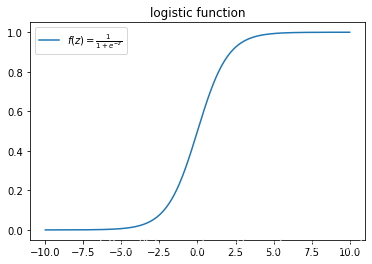
先来看一下logistic回归函数长啥样?

from scipy.special import expit #导入logistic函数
myx = np.linspace(-10, 10, 1000) #自变量
myy = expit(myx)
plt.plot(myx, myy, label = r"$f(z)=\frac{1}{1+e^{-z}}$")
plt.legend()
plt.title("logistic function")

logistic

原数据

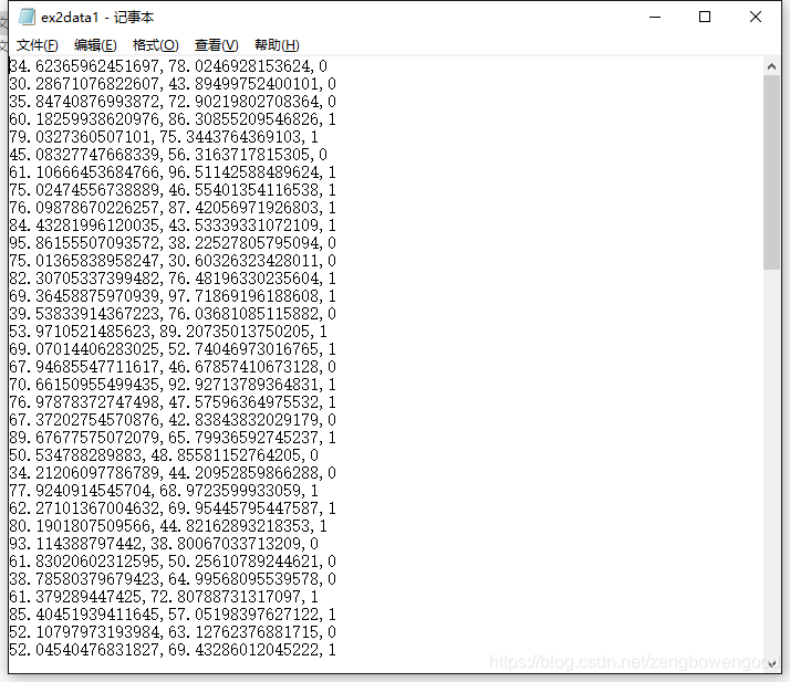
原数据是关于某小学生考试的语文成绩和数学成绩以及是否被录取的资料。请忽略小数点后几位数，如果需要数据可以来“三行科创”微信公众号交流群索要。

数据处理和探索

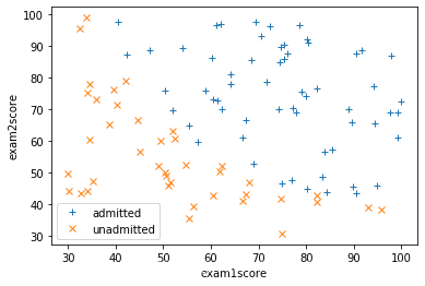
有了数据就需要进行一系列探索，这里隔离出特征和标签，以及数据可视化

import numpy as np
import pandas as pd 
import matplotlib.pyplot as plt 
data = pd.read_csv("CourseraML/ex2/data/ex2data1.txt", header = None, names = ['exam1score', 'exam2score', 'label']) #读取数据
X = np.array(data[['exam1score','exam2score']]) #特征
y = np.array(data['label']) #标签
m = len(X) #样本量
X = np.insert(X, 0, 1, axis=1) #加上虚拟特征“1”
pos = np.array([X[i] for i in range(len(X)) if y[i] ==1]) #正性特征
neg  = np.array([X[i] for i in range(len(X)) if y[i]==0]) #负性特征

def dataPlot(): #定义数据可视化函数
    plt.figure(figsize = (6,4)) #新建画布
    plt.plot(pos[:,1], pos[:,2], "+", label = "admitted") #正性散点图
    plt.plot(neg[:,1], neg[:,2], "x", label = "unadmitted") #负性散点图
    plt.xlabel("exam1score")
    plt.ylabel("exam2score")
    plt.legend()
    
dataPlot()

散点图

假设函数，损失函数和最优化

从散点图大致可以看出两类数据还有有比较明显的区别的，需要找一个决策函数来判定

def h(mytheta, myX): #定义假设函数 
    return expit(np.dot(myX, mytheta)) 

def costFunction(start_theta, X, y, mylambda = 0): #定义损失函数
    term1 = np.dot(-np.array(y).T, np.log(h(start_theta, X))) 
    term2 = np.dot(-np.array(1-np.array(y)).T, np.log(1-h(start_theta, X)))
    regterm = (mylambda/2)*(np.sum(np.dot(start_theta.T, start_theta))) #正则项
    return float((1./m)*(term1 + term2 + regterm))
    
initial_theta = np.zeros((X.shape[1], 1)) #初始化theta值
print(costFunction(initial_theta, X, y, mylambda = 0))

from scipy import optimize

def optimizeTheta(_theta, _X, _y, mylambda = 0): #定义最优化函数
    result = optimize.fmin(costFunction, x0 = theta, args = (_X, _y, mylambda), maxiter = 400, full_output = True)
    return result[0], result[1]

print(optimizeTheta(initial_theta, X, y))
#https://docs.scipy.org/doc/scipy-0.16.0/reference/generated/scipy.optimize.fmin.html

输出为 (array([-25.16130062, 0.20623142, 0.20147143]), 0.20349770159021519)

决策函数

在获的最有参数之后就可以把决策函数表示出来，在低维情况下还可以可视化决策函数

theta, mincost = optimizeTheta(initial_theta, X, y)

boundary_xs = np.array([np.min(X[:,1]), np.max(X[:,1])]) #决策边界的自变量
boundary_ys = (-1./ theta[2])*(theta[0]+theta[1]*boundary_xs)
dataPlot()
plt.plot(boundary_xs, boundary_ys, "b-", label = "decision boundary")
plt.legend()

决策函数

混肴矩阵

混肴矩阵主要用来评判分类模型的好坏，是最基本的评价指标

def makeDecision(mytheta, myX): #定义决策函数构造混肴矩阵
    label_pred = np.zeros(len(myX)) #初始化预测值组
    for i in range(len(myX)):
        if h(mytheta, myX[i,:]) >= 0.5:
            label_pred[i]= 1
        else:
            label_pred[i]= 0
    return label_pred.T

y_pred = makeDecision(theta, X).T

from sklearn.metrics import confusion_matrix    #引入混肴矩阵
tn, fp, fn, tp  = confusion_matrix(y, y_pred).ravel() #调用ravel()来直接得到这四个值
print(tn, fp, fn, tp)
plt.matshow([[tn, fp], [fn, tp]])
plt.title('Confusion matrix')
plt.colorbar()
plt.ylabel('True label')
plt.xlabel('Predicted label')
plt.show()

混肴矩阵

ROC曲线
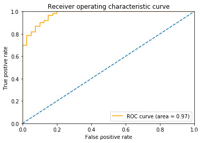
除了最基本的混肴矩阵，ROC曲线更被人们使用

from sklearn.metrics import roc_curve, auc
y_true = np.array(y) #真实标签
y_score = np.array(h(theta, X)) #预测概率
fpr, tpr, thresholds= roc_curve(y_true, y_score)
roc_auc = auc(fpr,tpr)

plt.figure(figsize = (6,4))
plt.plot(fpr, tpr, color = 'orange', label = "ROC curve (area = %0.2f)"% roc_auc)
plt.plot([0,1], [0,1], linestyle = '--')
plt.xlim([0, 1])
plt.ylim([0, 1])
plt.xlabel("False positive rate")
plt.ylabel("True postive rate")
plt.title("Receiver operating characteristic curve")
plt.legend()

roc曲线
延伸阅读

机器学习——多元线性回归模型
 机器学习——单变量线性回归模型

在这里插入图片描述

机器学习——逻辑回归基础

猜你喜欢