感谢:
https://blog.csdn.net/lu597203933/article/details/38468303
https://www.bilibili.com/video/av10590361/?p=31&t=176 logistic regression chapter
以及《机器学习实战》 第五章
'''
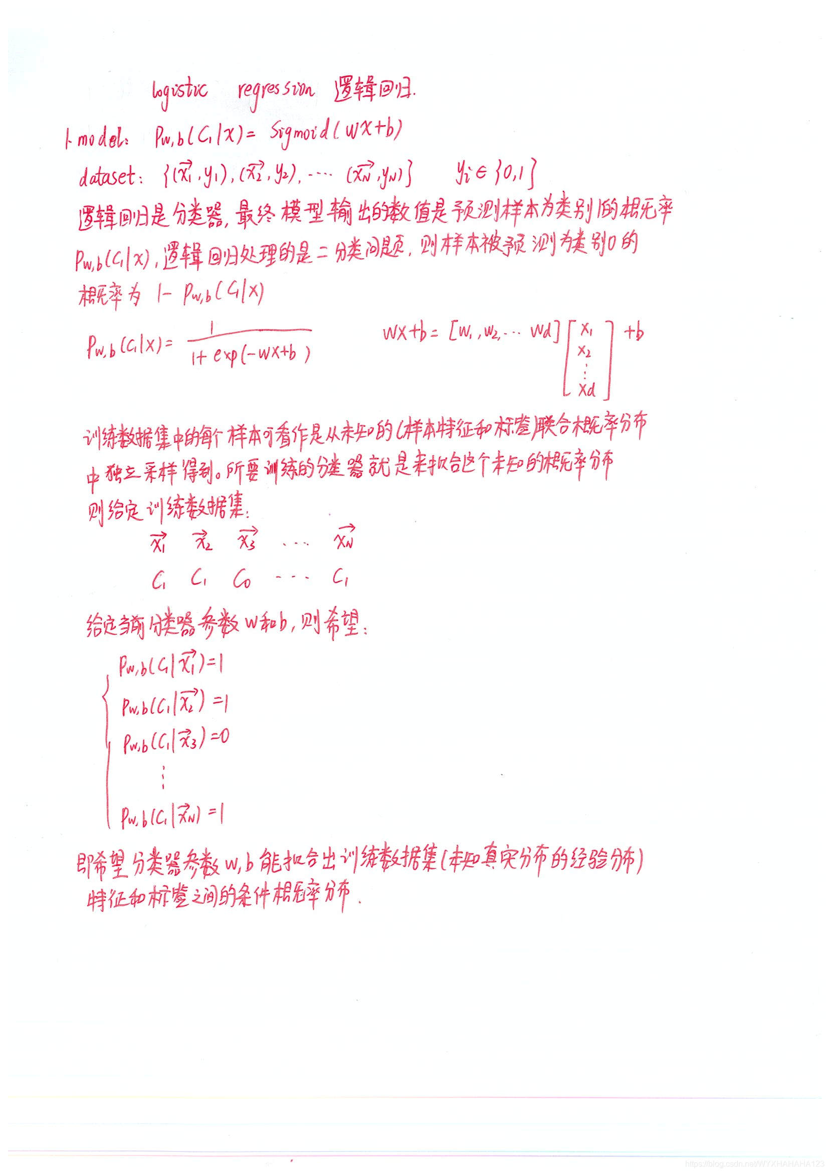
logistic regression 逻辑回归:实际上是分类问题
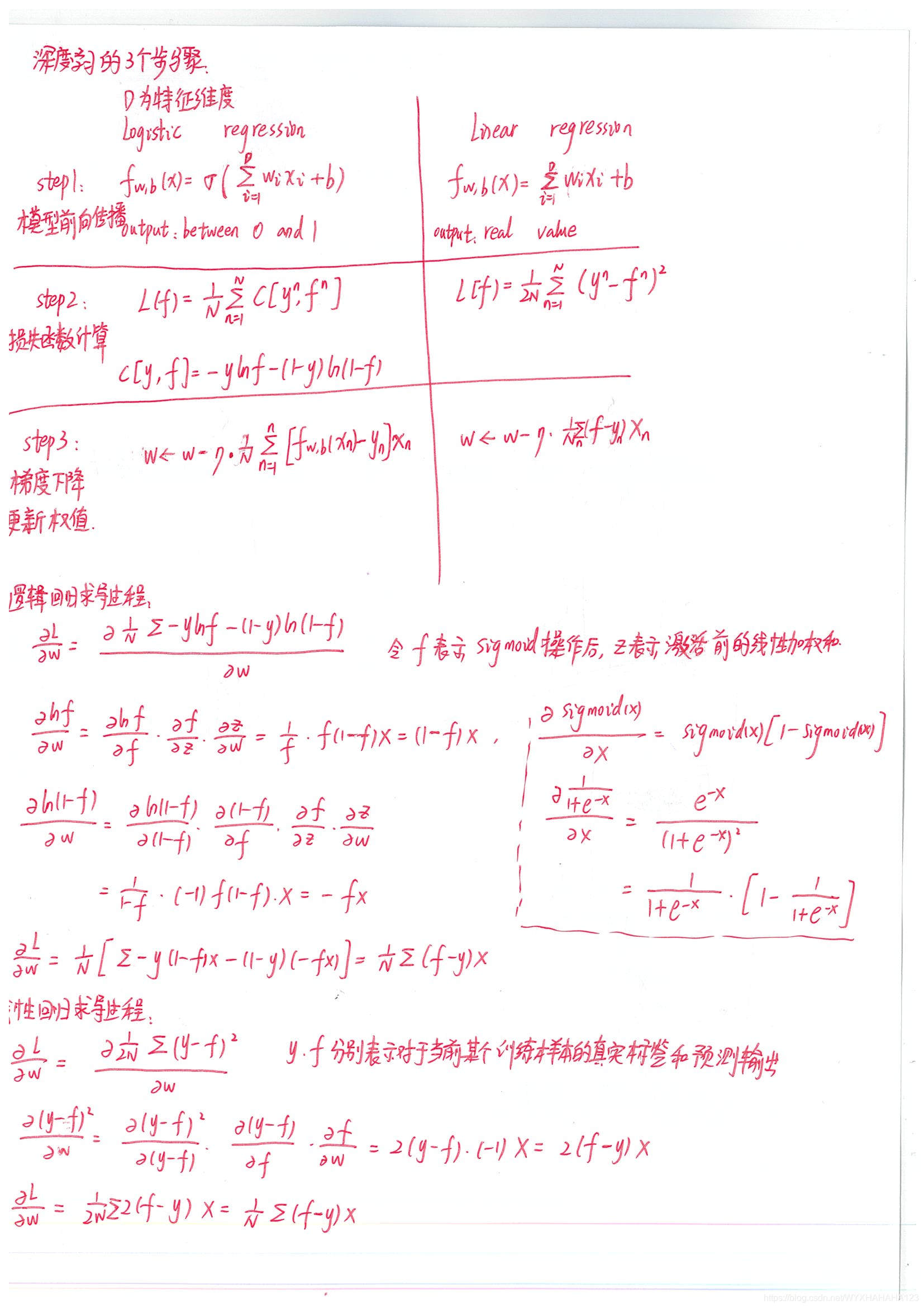
梯度下降算法找到loss损失函数的最小值点
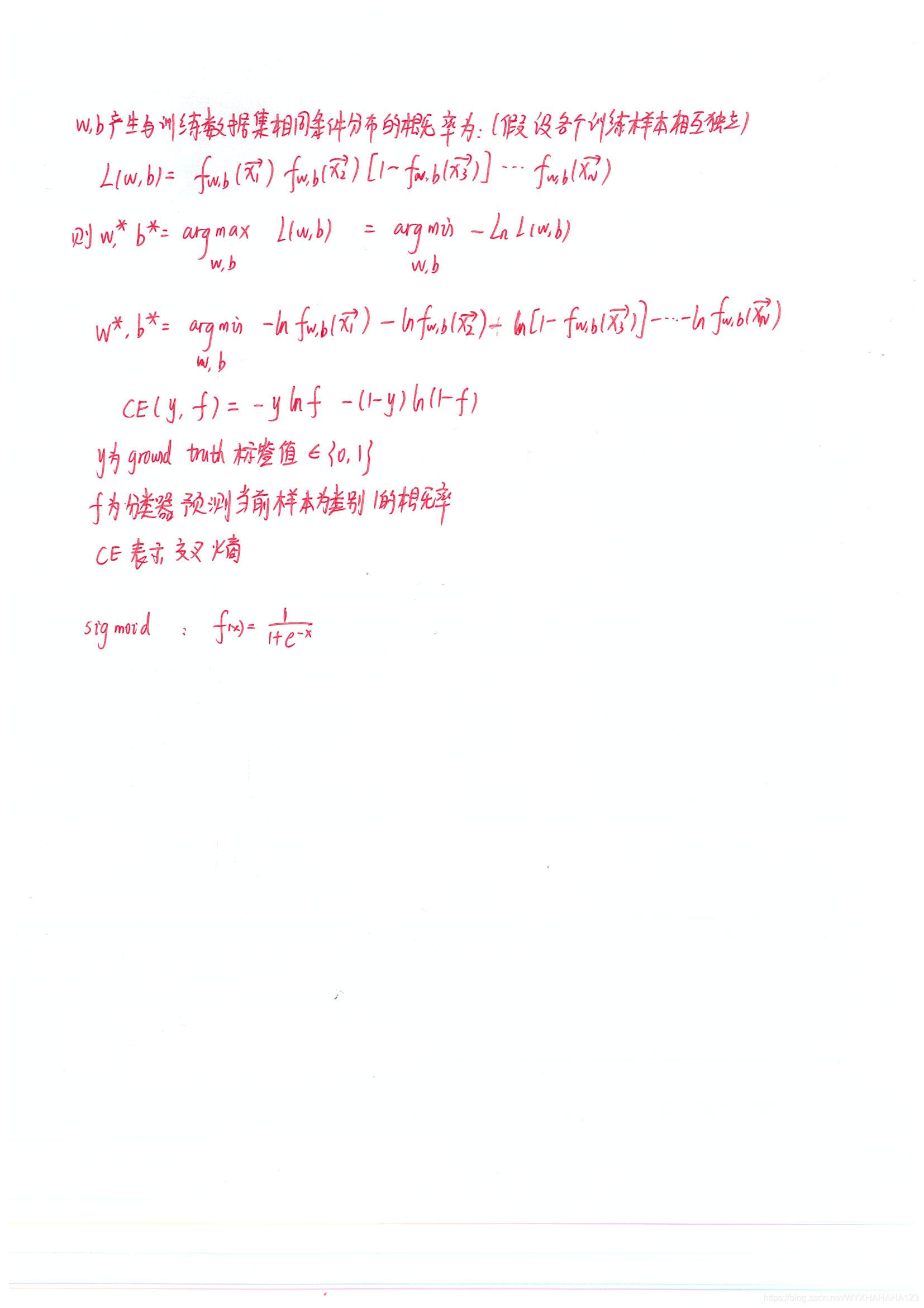
逐步迭代,找到最佳的回归系数,逻辑回归的分类器模型参数更新的过程就是
模型学习/训练的过程,也可以理解成是模型最佳系数回归的过程
'''
import numpy as np
import os
import matplotlib.pyplot as plt
import random
def Read_Data(data_path):
'''
读取所给出的保存数据的完整txt路径,并转换成对应的numpy数组
:param data_path:
:return:
'''
file_obj=open(data_path)
all_lines=file_obj.readlines()
num_samples=len(all_lines)
num_feat=len(all_lines[0].split())-1
data_array=np.zeros((num_samples,num_feat))
label_array=np.zeros((num_samples))
# print(data_array.shape)
for i,line in enumerate(all_lines):
line=line.split()
for j in range(num_feat):
if line[j][0]=='-':
data_array[i][j]=-float(line[j][1:])
else:
data_array[i][j]=float(line[j])
label_array[i]=int(line[-1])
file_obj.close()
return data_array,label_array
class logistic_reg(object):
def __init__(self,num_feat):
# self.weight=np.random.rand(num_feat).reshape(num_feat,1)
self.weight = np.ones(num_feat).reshape(num_feat, 1)
# self.bias=np.ones((1))
def forward(self,train_data,train_label,lr,is_training):
# 根据前向传播计算得到的对于训练数据的预测值和训练数据标签,求出损失函数,并更新
# 模型的参数
'''
:param train_data: numpy.array = [num_samples,num_feat]
:return:
'''
# train_data=np.concatenate((train_data,np.ones((train_data.shape[0],1))),axis=1)
train_data=np.concatenate((np.ones((train_data.shape[0],1)),train_data),axis=1)
pred=np.dot(train_data,self.weight)
# pred shape [num_samples,1]
pred=1+np.exp(-pred)
pred=1/pred
# 前向传播,计算在当前模型的回归参数下,所预测的输出
if not is_training:# 在评估模式下,直接返回模型所预测的概率值
return pred
else:
log_fore=-np.log(pred)# 对于ground truth label为1的样本
log_back=-np.log(1-pred)
if len(train_label.shape)==1:
train_label=np.expand_dims(train_label,axis=1)
loss=np.sum(log_fore[np.where(train_label==1)])+np.sum(log_back[np.where(train_label==0)])
loss/=train_data.shape[0]
# 损失函数计算结束
# 梯度下降算法
error=pred-train_label
dW=np.dot(train_data.T,error)
# dW = [num_feat,1]
# dW/=train_data.shape[0]
db=np.mean(pred-train_label)
self.weight-=lr*dW
# self.bias-=lr*db
return pred,loss
if __name__=='__main__':
data_root_path='F:\\machine_learning\\Ch05'
data_path=os.path.join(data_root_path,'testSet.txt')
data_array,label_array=Read_Data(data_path)
# print(data_array,label_array)
# print(data_array.shape)
log_model=logistic_reg(data_array.shape[1]+1)
epoch=500
lr=0.001
for i in range(epoch):
pred,loss=log_model.forward(data_array,label_array,lr,is_training=True)
# print('epoch',i,'loss',loss)
print('weight',log_model.weight)
# print('bias',log_model.bias)
print(pred.shape,np.min(pred),np.max(pred))
prediction=np.where(pred>0.5,1,0)
prediction=prediction.reshape(-1)
# print(prediction[:50])
# print(label_array[:50])
accuracy=np.sum(prediction==label_array)/label_array.shape[0]
print('full batch training , accuracy',accuracy)
'''
使用梯度下降法,每次迭代/更新梯度值使用的是整个训练数据集
即一次处理的是所有的数据,称为批处理
accuracy 0.96
'''
# [[ 0.82234723]
# [-0.27227592]
# [ 1.03490603]]
fig = plt.figure()
ax1 = fig.add_subplot(111)
# 设置标题
ax1.set_title('two dimension data')
# 设置X轴标签
plt.xlabel('x0')
# 设置Y轴标签
plt.ylabel('x1')
# 画散点图
fore_point=data_array[np.where(label_array==1)]
back_point=data_array[np.where(label_array==0)]
ax1.scatter(x=fore_point[:, 0], y=fore_point[:, 1], c='r', marker='o')
# 设置图标
plt.legend('fore_point')
ax1.scatter(x=back_point[:, 0], y=back_point[:, 1], c='b', marker='^')
# 设置图标
plt.legend('back_point')
x=np.arange(-3,3,0.1)
y=-(log_model.weight[1]/log_model.weight[2])*x-(log_model.weight[0]/log_model.weight[2])
plt.scatter(x,y,c='g', marker='.')
# 显示所画的图
plt.show()
'''
批量的梯度下降法(每更新一次回归系数,需要使用到训练数据集中的所有数据)对于大规模数据集的处理计算复杂度会很高
故而引入随机梯度下降法
随机梯度下降法:每次使用一个训练样本计算得到的梯度值更新回归系数,称为在线学习
随机梯度下降法可以看作是batch size=1的mini-batch梯度下降法,深度学习中通常的做法是:
对于每个epoch,首先将整个训练数据集的数据进行随机重排(random shuffle),然后在每个step中从
随机重排后的数据集中采样出batch size个样本,更新一次回归系数,再进行下一个step的操作,
对于同一个epoch而言,每个step采样出来的样本是不具有overlap的,而同一个epcoh的所有step
所使用到的样本总数就是整个训练数据集
在这里的小批量梯度下降算法中,引入polynomial learning rate,即在训练过程中,学习率呈现多项式曲线的下降趋势
lr(t)=base_lr*(t/T)**power
t表示当前step步数,T表示总的step步数
'''
log_model_2 = logistic_reg(data_array.shape[1] + 1)
epoch = 50
lr=0.1
# base_lr = 0.1
batch_size=1
if data_array.shape[0]%batch_size==0:
num_step=data_array.shape[0]//batch_size
else:
num_step = int(data_array.shape[0]/ batch_size)+1
# T = epoch * num_step
for i in range(epoch):
# 在每个epoch开始时对整个训练数据集进行随机重排
index=random.sample(range(data_array.shape[0]), data_array.shape[0])
if i%25==0:
lr*=0.1
# print(i,lr)
for j in range(num_step):
# lr=base_lr*(num_step*i+j+1)/()
row_start=j*batch_size
row_end=(j+1)*batch_size
if row_end>data_array.shape[0]:
row_end=data_array.shape[0]
pred, loss = log_model_2.forward(data_array[index[row_start:row_end]], label_array[index[row_start:row_end]], lr, is_training=True)
# print('epoch',i,'loss',loss)
pred=log_model_2.forward(data_array,label_array,lr=0,is_training=False)
prediction = np.where(pred > 0.5, 1, 0)
prediction = prediction.reshape(-1)
accuracy = np.sum(prediction == label_array) / label_array.shape[0]
print('mini batch accuracy', accuracy)
# print('weight', log_model.weight)
# print('bias',log_model.bias)
# mini batch accuracy 0.96 经过50次遍历,可达到与梯度下降法遍历500次相同的准确率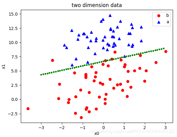
    '''
    读取真实数据即大规模数据集
    '''
    data_root_path = 'F:\\machine_learning\\Ch05'
    data_path = os.path.join(data_root_path, 'testSet.txt')
    data_train,label_train=Read_Data(os.path.join(data_root_path,'horseColicTraining.txt'))
    data_test,label_test=Read_Data(os.path.join(data_root_path,'horseColicTest.txt'))
    print(data_train.shape,label_train.shape)

    # (299, 21) (299,)   数据集中的训练样本含有21维的特征

    horse_model=logistic_reg(num_feat=data_train.shape[1]+1)

    epoch = 50
    lr=0.1
    # base_lr = 0.1
    batch_size=50
    if data_train.shape[0]%batch_size==0:
        num_step=data_train.shape[0]//batch_size
    else:
        num_step = int(data_train.shape[0]/ batch_size)+1
    # T = epoch * num_step
    for i in range(epoch):
        # 在每个epoch开始时对整个训练数据集进行随机重排
        index=random.sample(range(data_train.shape[0]), data_train.shape[0])
        if i%25==0:
            lr*=0.1
        # print(i,lr)
        for j in range(num_step):
            # lr=base_lr*(num_step*i+j+1)/()
            row_start=j*batch_size
            row_end=(j+1)*batch_size
            if row_end>data_train.shape[0]:
                row_end=data_train.shape[0]
            pred, loss = horse_model.forward(data_train[index[row_start:row_end]], label_train[index[row_start:row_end]], lr, is_training=True)
            # print('epoch',i,'loss',loss)
        pred=horse_model.forward(data_test,label_test,lr=0,is_training=False)
        prediction = np.where(pred > 0.5, 1, 0)
        prediction = prediction.reshape(-1)

        accuracy = np.sum(prediction == label_test) / label_test.shape[0]
        print('epoch',i,'horse mini batch accuracy', accuracy)
        '''
        epoch 48 horse mini batch accuracy 0.7611940298507462
        epoch 49 horse mini batch accuracy 0.7014925373134329
        '''