

CVPR-2019
文章目录
1 Background and Motivation
随着深度学习技术的发展,image classification 的精度也越来越高!
精度的提升不仅仅来自于 model architecture,也来自如下的 training procedure refinements
- loss functions
- data pre-processing
- optimization methods
- learn rate schedule
- stride size of a particular convolution layer
然而 training procedure refinements 往往没有 model architecture 那样吸睛,都被冷落在论文中的 implementation details 部分 or only visible in source code
本文,作者翻牌 training procedure refinements

对各种 training procedure refinements 进行了详细的分析实验,通过组合拳,把 ResNet 在 ImageNet 上的 Top-1 ACC 从 75.3% 提到了 79.29%,这些技巧用在 object detection 和 semantic segmentation 任务中也能提升精度!

2 Advantages / Contributions
总结归纳各种 tricks,组合起来调 resnet,精度从 75.3 提到了 79.29(Top of ImageNet)

3 Baseline
提供了一种标准训练测试流程
训练
- 32-bit,0~255
- randomly crop,aspect ratio [3/4,4/3],scale [8%, 100%],最后 resize 到 224×224
- 50% 水平翻转
- hue,saturation,brightness 增强 [0.6,1.4](参考本博客附录部分)
- PCA noise(参考本博客附录部分)
- 减均值除以方差

测试
- resize 短边到 256,保持 aspect ratio,从中心区域中截选出 224×224
- 减均值除以方差
按照上述标准流程,得到的结果如下表所示

4 Efficient Training
4.1 Large-batch training
大 batch-size 的好处在于,会缩短训练时间
但是
For convex problems,convergence rate decreases as batch size increases
这里理解起来可能不是那么顺畅,再看看这个讨论(Rhett 的回答)

换句话说
for the same number of epochs,training with a large batch size(仅仅增大 batch-size,不做其他的改变) results in a modal with degraded validation accuracy compared to the ones trained with smaller batch sizes
想在不影响收敛速度(精度)的情况下,加快训练速度(增大batch),作者给出了如下的建议
1)Linear scaling learning rate

大的 batch-size 只会 reduce the noise in the gradient,并没有改变 expectation of stochastic gradient(个人感觉期望还是有改变的),因此采用大的 bath-size 后,可以采用大的学习率提升其收敛速度
eg:batch-size 为 256,采用 0.1 0.1 0.1 初始学习率
则:batch-size 为 b b b, 应该用 0.1 × b / 256 0.1 × b / 256 0.1×b/256
2)Learning rate warmup

训练刚开始时,参数都是随机初始化的,离 final solution 十万八千里,这个时候用太大的学习率容易导致 numerical instability
此时,比较好的处理方式时慢热,类似于热身,让网路通过几个 epoch 的学习后达到初始学习率
eg:初始学习率为 η \eta η,用 m m m 次 iteration 到初始学习率,那么第 i i i 次( 1 ≤ i ≤ m 1≤i≤m 1≤i≤m)迭代的学习率应该为 i η / m i \eta /m iη/m
下图最左边部分即为 warmup

3)Zero γ \gamma γ

ResNet 的 bottleneck 部分可以表示为 X + F ( x ) X + F(x) X+F(x),

在每个 bottleneck 中, F ( x ) F(x) F(x) 以是以 batch-normalization 层结束的,batch-normalization 算法如下图所示(详细解析可以参考 【BN】《Batch Normalization: Accelerating Deep Network Training by Reducing Internal Covariate Shift》)

常规操作中, γ \gamma γ 和 β \beta β 初始化的值分别为 1 和 0,也即 X + 1 × F ( x ) + 0 X + 1×F(x) + 0 X+1×F(x)+0
Zero γ \gamma γ 策略中, γ \gamma γ 的初始化为 0,也即 X + 0 × F ( x ) + 0 X + 0×F(x) + 0 X+0×F(x)+0, F ( x ) F(x) F(x) 部分直接被砍了,仅返回 X X X
all residual blocks just return their inputs,mimics network that has less number of layers and is easier to train at the initial stage.
4)No bias decay

正常情况下,weight-decay 会应用到 all learnable parameters,包括 weight,bias, batch normalization 算法中的 γ \gamma γ 和 β \beta β!
目的是进行 L2 regularization,drives their values towards 0
但 weight-decay 一般时为了防止过拟合才使用
在 no bias decay heuristic 中,除了 weight 用 weight-decay,其他的 learnable parameters 都没有使用 weight-decay!包括 batch normalization 算法中的 γ \gamma γ 和 β \beta β
4.2 Low-precision training
New hardware, however, may have enhanced arithmetic logic unit for lower precision data types
比如 V100 显卡,32 bit 浮点运算提供 14T FLOPS,16 bit 浮点运算提供 over 100T FLOPS!算力越多,可以承载的运算量更大

上表展示了在不同算力下的结果(256 batch-size vs 1024 batch-size,还引入了 linear scaling learning rate 策略)
可以看出,低精度不仅加速,效果还很猛
下面看看 16bit 的代码实现
16bit 精度是将内存占用减半的惊人技术。大多数模型使用 32bit 精度数字进行训练。然而,最近的研究发现,16bit 模型也可以工作得很好。
混合精度意味着对某些内容使用16bit,但将权重等内容保持在 32bit。
要在Pytorch中使用16bit 精度,请安装NVIDIA的apex库,并对你的模型进行这些更改。
# enable 16-bit on the model and the optimizer
model, optimizers = amp.initialize(model, optimizers, opt_level='O2')

# when doing .backward, let amp do it so it can scale the loss
with amp.scale_loss(loss, optimizer) as scaled_loss:
    scaled_loss.backward()
amp包会处理好大部分事情。如果梯度爆炸或趋向于0,它甚至会缩放loss。
英文原文:
9 Tips For Training Lightning-Fast Neural Networks In Pytorch
中文翻译:
9个技巧让你的PyTorch模型训练变得飞快!
但是要小心一些不安全的操作如 mean 和 sum,溢出fp16。(Pytorch有什么节省显存的小技巧? - 郑哲东的回答 - 知乎)
4.3 Experiment Results

感觉应该是每行单独加上第一行的结果,而不是累加的结果,可以看出,作者引出的 tricks 还是蛮实在的
PS:如果是累加的结果,感觉 No bias decay 的意义就失去了
5 Model Tweaks
5.1 ResNet Architecture
先看看 ResNet 原论文中的结构,注意 50-layer 这一列

下面看看作者对原始结构的描述

5.2 ResNet Tweaks
在实践和理论发展过程中,resnet 不断优化
1)ResNet-B
改进前 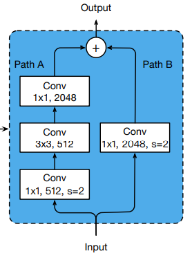 改进后
改进后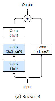
在 Figure1 的 Down sampling 模块中,Path A 一上来就用 1×1 步长为 2 的 conv,会导致信息损失 3/4,
ResNet-B 在 ResNet-A 的基础上,将步长为 2 的操作后移到了 3×3 conv 中(3×3 配合步长 2 是会遍历到原始特征图所有空间位置的,所以很大程度上弥补了信息损失),一定程度上平滑了信息的过渡阶段
2)ResNet-C
改进前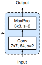 改进后
改进后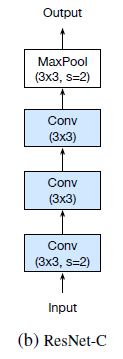
在 Figure1 的 Input stem 模块中,采用的是 7×7 Conv
后续学者们发现,computational cost 与卷积核的大小是 quadratic 关系,所以 7×7 Conv ~5.4(49/9 ) more expensive than 3×3 Conv
为了效率,把 7×7 Conv 换成了 3 个 3×3 Conv
3)ResNet-D
改进前 改进后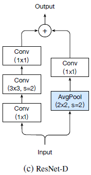
ResNet-B 结构基于 ResNet 中 path A 分支的不足进行了改进,作者进一步指出,path B 也出现了 1×1 Conv 搭配步长为 2,也会导致 3/4 information 流失,因此引入 average pooling 来缓解信息的流失,如 figure 2(C)所示
5.3 Experiment Results

这里 ResNet-C 包含了 ResNet-B 的 tweaks,ResNet-D 包含了 ResNet-B 和 ResNet-C 的 tweaks
模型 B 到 C 的变换中, 可以观察到 FLOPs 增加了,作者这里应该是改变了 3 个 3× 3 Conv 的 channels,如果保持和 7×7 一样的话,FLOPs 是会减少的
6 Training Refinements
6.1 Cosine Learning Rate Decay

t t t 表示 t t t-th bath,T 表示训练中所有 batch 的数量(这里 batch 可以理解为 epoch), η \eta η 是初始的学习率
上面公式 cos 里的范围为 0 0 0~ π \pi π,cos 的范围为 1 1 1 ~ − 1 -1 −1,加上外面的 1 然后除以 2 范围为 1 1 1 ~ 0 0 0,最后 × η \eta η,可以看出上述公式是在初始学习率的基础上,以 cos 函数的走势,降到 0,也即 cosine decay
下图展示了 warmup 和 cosine decay 策略

相比于 step decay,一开始下降比较快,后面缓慢下降
下面自己实现下公式(1)
import matplotlib.pyplot as plt
import numpy as np

T = 120
x = np.arange(T)

lr = 0.01
y1 = 1/2 * (1+ np.cos(np.pi * x / T)) * 0.01   # cosine decay

y2 = [0.01]*30 + [0.001]*30 + [0.0001]*30 + [0.00001]*30  # step decay

plt.plot(x, y1)
plt.plot(x, y2, "--")
plt.show()

6.2 Label Smoothing
原理可以参考 【Inception-v3】《Rethinking the Inception Architecture for Computer Vision》
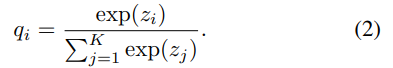
softmax 的输出 q q q
原始 GT 分布为
p i = { 1 i = y 0 i ≠ y p_i = \left\{\begin{matrix} 1 & i=y\\ 0 & i\neq y \end{matrix}\right. pi={ 10i=yi=y
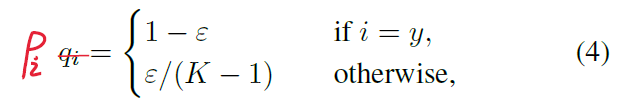
label smoothing 后的 GT 分布 p p p
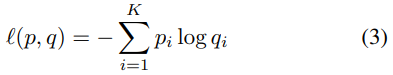
交叉熵损失
原始输出最优解(导数为 0 时)为
z i ∗ = i n f z_i^* = inf zi∗=inf
缺点是太自信了
it encourages the output scores dramatically distinctive which potentially leads to overfitting
引入 label smoothing 后的最优解为
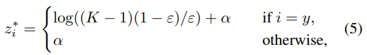
求导细节可以参考 label smoothing 如何让正确类与错误类在 logit 维度拉远的?
图 4 (a)展示了 K = 1000 K=1000 K=1000 时,最优解 z i ∗ z_i^* zi∗ 随着 ϵ \epsilon ϵ 的变化的趋势

自己画画试试
import matplotlib.pyplot as plt
import numpy as np

K = 1000
x = np.arange(0.01, 1.0, 0.01)
y = np.log2((K-1)*(1-x)/x)
plt.plot(x, y)
plt.show()

图(b) 展示的是加 label smooth 和不加 label smooth 时, the gap between the maximum prediction and the average of the rest

可以看到引入 label smoothing 后,with label smoothing the distribution centers at the theoretical value and has fewer extreme values
GT 类和其他类预测的结果差距变小了(没那么自信了),而且比较集中,跨度没有那么大(优化空间减少了)
我们也可以看看理论的峰值
import math
K = 1000
alpha = 4  # 这里比较随意
x = 0.1
diff = math.log((K-1)*(1-x)/x, math.e) + alpha - alpha
print(diff)
output
9.103979355984773
和图中蓝色虚线峰值的横坐标相呼应
6.3 Knowledge Distillation
【Distilling】《Distilling the Knowledge in a Neural Network》
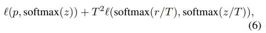
z z z 和 r r r 分别为 student model 和 teacher model 的 logits
T T T 是温度
6.4 Mixup Training
randomly sample two examples,然后 weighted linear interpolation of these two examples
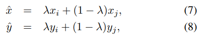
λ \lambda λ~ B e t a ( α , α ) Beta(\alpha,\alpha) Beta(α,α) 分布

使用时要配合更多的 epochs
increase the number of epochs from 120 to 200 because the mixed example ask for longer training progress to converge better
6.5 Experiment Results

Teacher 网络是 ResNet-152-D
Teacher 网络也使用了 cosine decay / label smoothing / mixup( α = 0.2 \alpha=0.2 α=0.2)
观察到知识蒸馏在 Inception 和 mobilenet 上的表现并不是很好,作者的解释为
Our interpretation is that the teacher model is not from the same family of the student, therefore has different distribution in the prediction, and brings negative impact to the model.
在 MIT Places365 data-set 上验证一下泛化性,结果如下所示

7 Transfer Learning
7.1 Object Detection

基于 Faster RCNN 框架,在 VOC 数据集上训练测试,结果如 Table 8 所示
第一列是在 ImageNet 的上的训练结果
7.2 Semantic Segmentation
基于 FCN 框架,在 ADE20K 上进行结果评估

cosine decay 依然坚挺,

其他策略就疲软了! 作者相应的解释为
semantic segmentation provides dense prediction in the pixel level. While models trained with label smoothing, distillation and mixup favor soften labels, blurred pixel-level information and degrade overall pixel-level accuracy.
8 Conclusion(own)
- 行文结构更像是实验报告,或者毕业论文
- 大 batch-size 和大 learning rate 配对
- 初始化 BN 层的参数都为 0
- 仅权重做 weight decay
- warm up
- 16 bit
- conv 1×1 配合 stride = 2,会丢失 3/4 的 information
- Cosine Learning Rate Decay
- Label Smoothing
- Knowledge Distilling
- Mixup
- 截取一下大 batchsize 的缺点
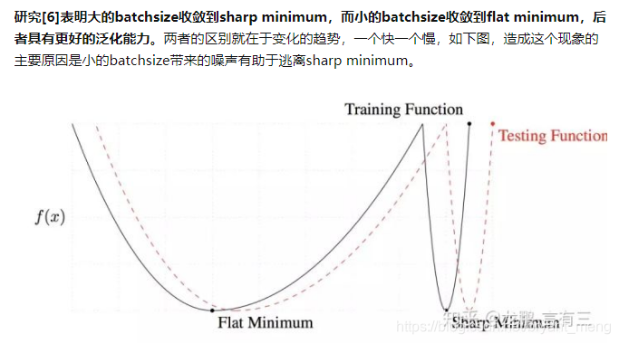
深度学习中的batch的大小对学习效果有何影响? - 言有三的回答 - 知乎
https://www.zhihu.com/question/32673260/answer/675161450
【附录】
hue,saturation,brightness 数据增强
来自 SSD中的数据增强细节


PCA noise 数据增强方式
来自 《ImageNet Classification with Deep Convolutional Neural Networks》,也即 AlexNet,核心公式为

-
λ \lambda λ 和 p ⃗ \vec{p} p 为协方差矩阵(3 × 3 covariance matrix of RGB pixel values)的特征值和特征向量
-
α \alpha α 是根据高斯分布产生的系数
具体实现如下,参考 【方法】数据增强(Data Augmentation)
import numpy as np
from PIL import Image
import random

import matplotlib.pyplot as plt

def pca_jitter(image_path):
    img = Image.open(image_path)
    img = np.asanyarray(img, dtype="float32")
    img = img / 255.0 # 0~1 之间
    img1 = img.reshape(img.size//3, 3)  # H*W*C to HW*C
    img1 = np.transpose(img1) # 转置
    img_cov = np.cov([img1[0], img1[1], img1[2]])  # covariance matrix
    lamda_cov, p_cov = np.linalg.eig(img_cov)  # eigenvector and eigenvalue of covariance matrix
    p_cov = np.transpose(p_cov)  # eigenvector

    alpha1 = random.gauss(0, 3) # 均值为0,方差为 3
    alpha2 = random.gauss(0, 3)
    alpha3 = random.gauss(0, 3)

    v = np.transpose((alpha1*lamda_cov[0], alpha2*lamda_cov[1], alpha3*lamda_cov[2])) # 核心公式

    add_num = np.dot(p_cov, v)

    img2 = np.array([img[:, :, 0] + add_num[0],
                     img[:, :, 1] + add_num[1],
                     img[:, :, 2] + add_num[2]])

    # bgr to rgb
    img2 = np.swapaxes(img2, 0, 2)
    img2 = np.swapaxes(img2, 0, 1)

    img2 = (img2-img2.min())/(img2.max()-img2.min()) # 归一化处理

    plt.subplot(1, 2, 1)
    plt.axis("off")
    plt.title("Original Image")
    plt.imshow(img)

    plt.subplot(1, 2, 2)
    plt.axis("off")
    plt.title("PCA jitter")
    plt.imshow(img2)
    plt.show()


pca_jitter("/home/Downloads/urban_beauty.jpg")
注意一些细节,
-
论文中 α \alpha α 从 N ∼ ( 0 , 0.1 ) N \sim (0,0.1) N∼(0,0.1) 高斯分布从产生,为了方便可视化效果,代码中的高斯分布为 N ∼ ( 0 , 3 ) N \sim (0,3) N∼(0,3)
-
原图加上 PCA 扰动后,像素值会溢出(超过 1 或者说超过 255),为了可视化方便,我进行了归一化处理(归一化到 0~1 之间),实际训练的时候不需要归一化
效果图如下:
