“吴恩达深度学习”第二周编程代码汇总（复现猫咪识别神经网络）

前言

这篇博客主要记录"吴恩达depplearning系列课程"第二周编程作业代码+自己的补充理解的相关内容，以作为学习记录。学习过程中借鉴了各位大佬的代码，想要追根溯源的朋友可以看这几位大佬的博客：大树先生的博客(英文版)，何宽（中文版）
作为初学者，本文的代码是自己当前能做到的”终极满意缝合怪“，同时部分原搬的代码也加了很多注释，便于理解。

目录

编程练习环境：Pycharm 2017.1/python 3.9

• 第1部分:使用Numpy的Python基础知识(可选赋值)，用numpy构建基本函数
  • 1.1 - sigmoid函数，np.exp()的一些前提介绍
  • 1.2 练习:使用numpy实现sigmoid函数
  • 1.3 sigmoid函数的梯度计算
  • 1.4 数组维度的重塑
  • 1.5 规范化矩阵的行
  • 1.6 广播（Broadcasting ）和softmax功能
• 第二部分：向量化
  • 2.1实现L1和L2损失函数
• 第三部分:逻辑回归与神经网络心态
  • 3.1 Packages
  • 3.2数据集的准备
• 第四部分:学习算法的一般架构
• 第五部分:构建神经网络（我们的算法部分
  • 5.1.辅助函数的使用
  • 5.2.初始化参数
  • 5.3.实现一个计算成本函数及其渐变的函数propagate（）
  • 5.4.优化
• 第六部分：将所有功能合并到一个模型中
• 第七部分：学习速率的选择
• 第八部分：用自己的图像测试
• 第九部分：完整代码

---

---

第一部分:使用Numpy的Python基础知识(可选赋值)，用numpy构建基本函数

介绍：
Numpy是Python中用于科学计算的主要包。它由一个大型社区(www.numpy.org)维护。在这个练习中，您将学习几个关键的numpy函数，如np.exp,np.log,和np.rehape。你需要知道如何在以后的作业中使用这些函数。

---

1.1 - sigmoid函数，np.exp()的一些前提介绍

尝试练习:
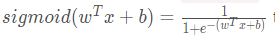
构建一个返回实数x的sigmoid的函数。可对指数函数使用math.exp(x)。
提示:

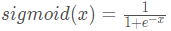
上述图片所示公式有时也被称为logistic函数。它是一个非线性函数，不仅用于机器学习(Logistic回归)，也用于深度学习。

当然，要引用属于特定包的函数，可以使用package_name.function()的形式调用它。运行下面的代码以查看math.exp()的示例。

# GRADED FUNCTION: basic_sigmoid
import math

def basic_sigmoid(x):
    """
    Compute sigmoid of x.
    
    Arguments:
    x -- A scalar

    Return:
    s -- sigmoid(x)
    """
    
    ### START CODE HERE ### (≈ 1 line of code)
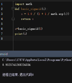
    s = 1.0 / (1 + 1/ math.exp(x))
    ### END CODE HERE ###
    
    return s

调用定义的函数basic_sigmoid(x)：

basic_sigmoid(3)

成功得到输出：

0.9525741268224334

实际上，我们在深度学习中很少使用“数学”库，因为函数的输入都是实数。但在深度学习中，我们主要使用矩阵和向量。这就是为什么numpy更有用。比如下例中我们就可以看出，对于实数成立的函数在矩阵的运用中就不再成功。

for example：

### One reason why we use "numpy" instead of "math" in Deep Learning ###
import math
def basic_sigmoid(x):
    s = 1.0 / (1 + 1 / math.exp(x))
    return s
x = [1, 2, 3]
a=basic_sigmoid(x)
print(a)

报错信息如下：

Traceback (most recent call last):
  File "D:\Adobe\PyCharm2017\lippractice\sigmoid.py", line 6, in <module>
    a=basic_sigmoid(x)
  File "D:\Adobe\PyCharm2017\lippractice\sigmoid.py", line 3, in basic_sigmoid
    s = 1.0 / (1 + 1 / math.exp(x))
TypeError: must be real number, not list

进程已结束,退出代码1

总而言之它试着告诉我们： basic_sigmoid(x) 运行失败是因为它需要接收的参数理想情况是一个实数，但我们传递进去的x[1,2,3]却是一个向量。
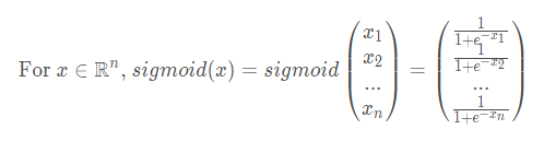
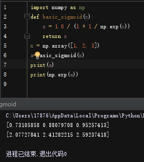
事实上，如果$ x = (x_1, x_2，…，x_n)$是一个行向量，那么函数np.exp(x)会将x包括的每一个元素映射到指数函数e^x上，结果将是：

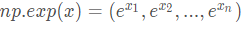
来看看代码运行就是：

import numpy as np
# example of np.exp
def basic_sigmoid(x):
    s = 1.0 / (1 + 1 / np.exp(x))
    return s
x = np.array([1, 2, 3])
a=basic_sigmoid(x)
print(a)
print(np.exp(a))# result is (exp(1), exp(2), exp(3))

输出结果：

[0.73105858 0.88079708 0.95257413]
[2.07727841 2.41282215 2.59237418]

此外，如果x是一个向量，那么进行一种Python运算时，例如s=x+3、s=x+ 3、s=1/x ；结果s将输出为与x大小相同的向量。

---

1.2 练习:使用numpy实现sigmoid函数

要求:
x可以是一个实数，一个向量，或者一个矩阵。我们在numpy中用来表示这些形状(向量、矩阵……)的数据结构称为numpy数组。你现在不需要知道更多。

代码如下：

# GRADED FUNCTION: sigmoid

import numpy as np # this means you can access numpy functions by writing np.function() instead of numpy.function()

def sigmoid(x):
    """
    Compute the sigmoid of x

    Arguments:
    x -- 任何大小的标量或numpy数组

    Return:
    s -- sigmoid(x)
    """
    
    ### START CODE HERE ### (≈ 1 line of code)
    s = 1.0 / (1 + 1 / np.exp(x))
    ### END CODE HERE ###
    
    return s

实际调用：

x = np.array([1, 2, 3])
sigmoid(x)

输出结果：

array([ 0.73105858,  0.88079708,  0.95257413])

练习结果：

---

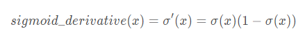
1.3 sigmoid函数的梯度计算

实现函数sigmoid_grad()来计算sigmoid函数关于其输入x的梯度。公式如下:

你通常用两步来编写这个函数:

1. 将s设为x的sigmoid型函数，你可能会发现sigmoid（x）很有用。
2. Compute σ ′ ( x ) = s ( 1 − s )
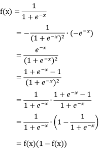
3. 补充一下2的证明过程：
   
   代码如下：

# GRADED FUNCTION: sigmoid_derivative
import numoy as np
def sigmoid_derivative(x):
    """
    Compute the gradient (also called the slope or derivative) of the sigmoid function with respect to its input x.
    You can store the output of the sigmoid function into variables and then use it to calculate the gradient.
    
    Arguments:
    x -- A scalar or numpy array

    Return:
    ds -- Your computed gradient.
    """
    
    ### START CODE HERE ### (≈ 2 lines of code)
    s = 1.0 / (1 + 1 / np.exp(x))
    ds = s * (1 - s)
    ### END CODE HERE ###
    
    return ds

实际调用：

x = np.array([1, 2, 3])
print ("sigmoid_derivative(x) = " + str(sigmoid_derivative(x)))

输出：

sigmoid_derivative(x) = [ 0.19661193  0.10499359  0.04517666]

练习结果：

---

1.4 重塑数组维度

简介：
深度学习中常用的两个numpy函数是np.shape和np.reshape()

• X.shape( )用于获得矩阵/向量X的形状(尺寸)。
• X. reshap( )被用来将X重塑成其他维度。

例如，在计算机科学中，图像是由三维形状数组表示的(length,height,depth=3)，depth=3是因为高度上包括Red(红)Green(绿)Blue(蓝)三个通道的数据。

然而，当您读取图像作为算法的输入时，您需要将其转换为一维的列向量：(length∗height∗3,1)

练习：
使用image2vector()，它接受一个维度为 (length, height, 3)的输入，然后返回一个维度为(length*height* 3,1)的矢量。
例如：
如果你想将一个数组（a，b，c）的维度 重塑为如(a*b,c)的矢量，你可以这样做:

v = v.reshape((v.shape[0]*v.shape[1], v.shape[2])) # v.shape[0] = a ; v.shape[1] = b ; v.shape[2] = c

请不要将图像的尺寸硬编码为常量（即不可更改）。相反，用image.shape[0]来查找你需要的数量，形状等。
代码如下：

# GRADED FUNCTION: image2vector
import numpy as np
def image2vector(image):
    """
    Argument:
    image -- a numpy array of shape (length, height, depth)
    
    Returns:
    v -- a vector of shape (length*height*depth, 1)
    """
    
    ### START CODE HERE ### (≈ 1 line of code)
    v = image.reshape((image.shape[0] * image.shape[1] * image.shape[2], 1))
    ### END CODE HERE ###
    
    return v

实际调用：

# This is a 3 by 3 by 2 array, typically images will be (num_px_x, num_px_y,3) where 3 represents the RGB values
image = np.array([[[ 0.67826139,  0.29380381],
        [ 0.90714982,  0.52835647],
        [ 0.4215251 ,  0.45017551]],

       [[ 0.92814219,  0.96677647],
        [ 0.85304703,  0.52351845],
        [ 0.19981397,  0.27417313]],

       [[ 0.60659855,  0.00533165],
        [ 0.10820313,  0.49978937],
        [ 0.34144279,  0.94630077]]])

print ("image2vector(image) = " + str(image2vector(image)))

输出结果：

image2vector(image) = [
 [ 0.67826139]
 [ 0.29380381]
 [ 0.90714982]
 [ 0.52835647]
 [ 0.4215251 ]
 [ 0.45017551]
 [ 0.92814219]
 [ 0.96677647]
 [ 0.85304703]
 [ 0.52351845]
 [ 0.19981397]
 [ 0.27417313]
 [ 0.60659855]
 [ 0.00533165]
 [ 0.10820313]
 [ 0.49978937]
 [ 0.34144279]
 [ 0.94630077]]

练习结果：

---

1.5 规范化矩阵的行

我们在机器学习和深度学习中使用的另一个常见技术是标准化我们的数据。它通常会带来更好的性能，因为梯度下降在归一化后收敛得更快。这里，通过规范化，我们的意思是求取x的范数(除以x的每个行向量的范数)。

例如,如果：

请注意，您可以划分不同大小的矩阵，它工作得很好:这被称为广播，您将在第5部分中学习它。
原理（即对于函数np.linalg.norm()的运用）：
linalg=linear（线性）+algebra（代数），norm则表示范数

x_norm=np.linalg.norm(x, ord=None, axis=None, keepdims=False)

1. x: 表示传入的矩阵（也可以是一维）
2. ord：范数类型
   
3. axis：处理类型
   axis=1表示按行向量处理，求多个行向量的范数
   axis=0表示按列向量处理，求多个列向量的范数
   axis=None表示矩阵范数。
4. keepdims：是否保持矩阵的二维特性
   True表示保持矩阵的二维特性，False相反

练习:自定义normalizeRows()函数来规范化矩阵的行。
要求：
将这个函数应用到输入矩阵x后，x的每一行都应该是一个单位长度的向量(意味该行每个元素的平方和开方的长度为1)。
代码如下：

# GRADED FUNCTION: normalizeRows
import numpy as np
def normalizeRows(x):
    """
    Implement a function that normalizes each row of the matrix x (to have unit length).
    
    Argument:
    x -- A numpy matrix of shape (n, m)
    
    Returns:
    x -- The normalized (by row) numpy matrix. You are allowed to modify x.
    """
    
    ### START CODE HERE ### (≈ 2 lines of code)
    # Compute x_norm as the norm 2 of x. Use np.linalg.norm(..., ord = 2, axis = ..., keepdims = True)
    x_norm = np.linalg.norm(x, axis=1, keepdims = True)  #计算每一行的长度，得到一个列向量
    
    # Divide x by its norm.
    x = x / x_norm  #利用numpy的广播，用矩阵与列向量相除。
    ### END CODE HERE ###

    return x

实例调用：

x = np.array([
    [0, 3, 4],
    [1, 6, 4]])
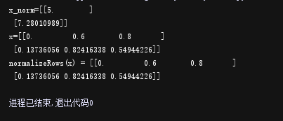
print("normalizeRows(x) = " + str(normalizeRows(x)))

输出结果：

normalizeRows(x) = [
 [ 0.          0.6         0.8       ]
 [ 0.13736056  0.82416338  0.54944226]]

练习展示：

注意:

在normalizeRows()中，您可以尝试打印x_norm和x的形状，然后重新运行评估。你会发现它们有不同的形状：
x_norm是（2，1）//两行一列
x是（2，3）//两行三列

这是正常的，因为x_norm取x的每一行的单位长度，所以x_norm有相同的行数，但是只有1列。那么当x除以x_norm时它是如何工作的呢?这就是广播（Broadcasting），我们现在就来谈谈!

---

1.6 广播（Broadcasting ）和softmax功能

在numpy中需要理解的一个非常重要的概念是“广播”。它对于在不同形状的数组之间执行数学运算非常有用。有关广播的全部细节，你可以阅读官方广播文件。
练习:使用numpy实现一个softmax函数。
要求：
当你的算法需要分类两个或更多的类时，你可以把softmax看作一个规格化函数。在本专业的第二门课程中，您将了解更多关于softmax的知识。
说明:

• Softmax回归函数是用于将分类结果归一化。但它不同于一般的按照比例归一化的方法，它通过对数变换来进行归一化，这样实现了较大的值在归一化过程中收益更多的情况。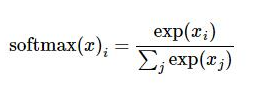
• 

代码如下：

# GRADED FUNCTION: softmax
import numpy as np
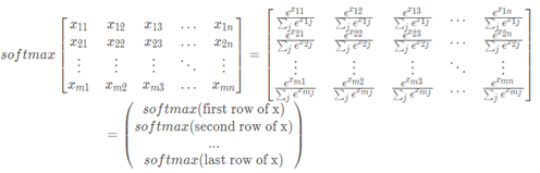
def softmax(x):
    """Calculates the softmax for each row of the input x.

    Your code should work for a row vector and also for matrices of shape (n, m).

    Argument:
    x -- A numpy matrix of shape (n,m)

    Returns:
    s -- A numpy matrix equal to the softmax of x, of shape (n,m)
    """
    
    ### START CODE HERE ### (≈ 3 lines of code)
    # Apply exp() element-wise to x. Use np.exp(...).
    x_exp = np.exp(x) # (n,m)

    # Create a vector x_sum that sums each row of x_exp. Use np.sum(..., axis = 1, keepdims = True).
    x_sum = np.sum(x_exp, axis = 1, keepdims = True) # (n,1)
    
    # Compute softmax(x) by dividing x_exp by x_sum. It should automatically use numpy broadcasting.
    s = x_exp / x_sum  # (n,m) 广播的作用

    ### END CODE HERE ###
    
    return s

实际调用：

x = np.array([
    [9, 2, 5, 0, 0],
    [7, 5, 0, 0 ,0]])
print("softmax(x) = " + str(softmax(x)))

输出结果：

softmax(x) = [[  9.80897665e-01   8.94462891e-04   1.79657674e-02   1.21052389e-04
    1.21052389e-04]
 [  8.78679856e-01   1.18916387e-01   8.01252314e-04   8.01252314e-04
    8.01252314e-04]]

注意:
如果你打印上面的x_exp、x_sum和s的形状，并重新运行评估单元格，你会看到x_sum是形状(2,1)，而x_exp和s是形状(2,5)。x_exp/x_sum工作是因为python广播。

你需要记住的:
np.exp(x)适用于任何np.array(x)并应用指数函数到每个坐标的sigmoid函数及其梯度-；image2vector是深度学习运算中常用的。np.reshape更被广泛应用。在未来，你将看到保持矩阵/向量的直线型将有助于消除许多bug。 numpy库有高效的内置函数，这体现了广播是非常有用的。

---

---

第二部分：向量化

在深度学习中，你要处理非常大的数据集。因此，一个非计算优化的函数可能成为你算法中的一个巨大瓶颈，并可能导致你的模型最终需要花费很长时间来运行。为了确保代码的计算效率，您将使用向量化。例如，试着说明dot/outer/elementwise乘积的下列实现之间的区别。（代码中重点关注dot/outer/elementwise对应的运行时长：）
注：

time.process_time()

返回当前进程的系统和用户CPU时间总和的值（以小数秒为单位）作为浮点数。
通常time.process_time()也用在测试代码时间上，根据定义，它在整个过程中。返回值的参考点未定义，因此我们测试代码的时候需要调用两次，做差值。
注意process_time()不包括sleep()休眠时间期间经过的时间。

代码比较：

import time
import numpy as np
x1 = [9, 2, 5, 0, 0, 7, 5, 0, 0, 0, 9, 2, 5, 0, 0]
x2 = [9, 2, 2, 9, 0, 9, 2, 5, 0, 0, 9, 2, 5, 0, 0]

### 经典向量点积的实现 ###
tic = time.process_time()#第一次时间获取
dot = 0
for i in range(len(x1)):#显示for循环控制运算
    dot+= x1[i]*x2[i]
toc = time.process_time()#第二次时间获取
print ("dot = " + str(dot) + "\n ----- Computation time = " + str(1000*(toc - tic)) + "ms")

### CLASSIC OUTER PRODUCT IMPLEMENTATION ###
tic = time.process_time()
outer = np.zeros((len(x1),len(x2))) # we create a len(x1)*len(x2) matrix with only zeros
for i in range(len(x1)):
    for j in range(len(x2)):
        outer[i,j] = x1[i]*x2[j]
toc = time.process_time()
print ("outer = " + str(outer) + "\n ----- Computation time = " + str(1000*(toc - tic)) + "ms")

### CLASSIC ELEMENTWISE IMPLEMENTATION ###
tic = time.process_time()
mul = np.zeros(len(x1))
for i in range(len(x1)):
    mul[i] = x1[i]*x2[i]
toc = time.process_time()
print ("elementwise multiplication = " + str(mul) + "\n ----- Computation time = " + str(1000*(toc - tic)) + "ms")

### CLASSIC GENERAL DOT PRODUCT IMPLEMENTATION ###
W = np.random.rand(3,len(x1)) # Random 3*len(x1) numpy array
tic = time.process_time()
gdot = np.zeros(W.shape[0])
for i in range(W.shape[0]):
    for j in range(len(x1)):
        gdot[i] += W[i,j]*x1[j]
toc = time.process_time()
print ("gdot = " + str(gdot) + "\n ----- Computation time = " + str(1000*(toc - tic)) + "ms")

输出结果：

dot = 278
 ----- Computation time = 0.2854390000002205ms
outer = [[ 81.  18.  18.  81.   0.  81.  18.  45.   0.   0.  81.  18.  45.   0.
    0.]
 [ 18.   4.   4.  18.   0.  18.   4.  10.   0.   0.  18.   4.  10.   0.
    0.]
 [ 45.  10.  10.  45.   0.  45.  10.  25.   0.   0.  45.  10.  25.   0.
    0.]
 [  0.   0.   0.   0.   0.   0.   0.   0.   0.   0.   0.   0.   0.   0.
    0.]
 [  0.   0.   0.   0.   0.   0.   0.   0.   0.   0.   0.   0.   0.   0.
    0.]
 [ 63.  14.  14.  63.   0.  63.  14.  35.   0.   0.  63.  14.  35.   0.
    0.]
 [ 45.  10.  10.  45.   0.  45.  10.  25.   0.   0.  45.  10.  25.   0.
    0.]
 [  0.   0.   0.   0.   0.   0.   0.   0.   0.   0.   0.   0.   0.   0.
    0.]
 [  0.   0.   0.   0.   0.   0.   0.   0.   0.   0.   0.   0.   0.   0.
    0.]
 [  0.   0.   0.   0.   0.   0.   0.   0.   0.   0.   0.   0.   0.   0.
    0.]
 [ 81.  18.  18.  81.   0.  81.  18.  45.   0.   0.  81.  18.  45.   0.
    0.]
 [ 18.   4.   4.  18.   0.  18.   4.  10.   0.   0.  18.   4.  10.   0.
    0.]
 [ 45.  10.  10.  45.   0.  45.  10.  25.   0.   0.  45.  10.  25.   0.
    0.]
 [  0.   0.   0.   0.   0.   0.   0.   0.   0.   0.   0.   0.   0.   0.
    0.]
 [  0.   0.   0.   0.   0.   0.   0.   0.   0.   0.   0.   0.   0.   0.
    0.]]
 ----- Computation time = 0.340502999999881ms
elementwise multiplication = [ 81.   4.  10.   0.   0.  63.  10.   0.   0.   0.  81.   4.  25.   0.   0.]
 ----- Computation time = 0.21034700000011064ms
gdot = [ 31.19670632  24.24358575  24.08807423]
 ----- Computation time = 0.4973530000000892ms

正如您可能已经注意到的，向量化的实现要干净得多，效率也更高。对于更大的向量/矩阵，运行时间的差异变得更大。
注意，np.dot()执行的是矩阵-矩阵或矩阵-向量的乘法。这与np.multiply()和*运算符(相当于Matlab/Octave中的.*)不同，后者只能执行元素的乘法。
练习结果：



值得关注的就是，计算出来的所有时间差都是0，猜测可能跟不同配置环境的运算速度有关；还有就是gdot数组结果明显不同，原因是因为W = np.random.rand(3,len(x1))是随机初始化的，所以结果只能近似。

---

2.1实现L1与L2的损失函数

练习:实现L1损失函数的numpy矢量化版本
你可能会发现函数abs(x) (x的绝对值)很有用。
提示:

• 损失函数用于评估模型的性能。你的损失越大，你的预测值yhat与真值y之间的差异就越大。在深度学习中，你可以使用梯度下降等优化算法来训练你的模型，并使成本最小化。
• L1的损失函数定义为：np.sum(np.abs(y - yhat))
  代码如下：

# GRADED FUNCTION: L1
import numpy as np
def L1(yhat, y):
    """
    Arguments:
    yhat -- vector of size m (predicted labels)
    y -- vector of size m (true labels)
    
    Returns:
    loss -- the value of the L1 loss function defined above
    """
    
    ### START CODE HERE ### (≈ 1 line of code)
    loss = np.sum(np.abs(y - yhat))
    ### END CODE HERE ###
    
    return loss

实际调用：

yhat = np.array([0.9, 0.2, 0.1, .4, .9])
y = np.array([1, 0, 0, 1, 1])
print("L1 = " + str(L1(yhat,y)))

输出结果：

L1 = 1.1

相当于就是：
loss =/0.9-1/+/0.2-0/+/0.1-0/+/0.4-1/+/0.9-1/
=0.1+0.2+0.1+0.6+0.1
=1.1

练习:实现L2损失的numpy矢量化版本。
有几种实现L2损失的方法，但您可能会发现函数np.dot()很有用。
代码如下：

# GRADED FUNCTION: L2
import numpy as np
def L2(yhat, y):
    """
    Arguments:
    yhat -- vector of size m (predicted labels)
    y -- vector of size m (true labels)
    
    Returns:
    loss -- the value of the L2 loss function defined above
    """
    
    ### START CODE HERE ### (≈ 1 line of code)
    loss =np.sum(np.power((y - yhat), 2))
    ### END CODE HERE ###
    
    return loss

实际调用：

yhat = np.array([.9, 0.2, 0.1, .4, .9])
y = np.array([1, 0, 0, 1, 1])
print("L2 = " + str(L2(yhat,y)))

输出结果：

L2 = 0.43

矢量化在深度学习中非常重要。它提供了计算效率和清晰度。而为了检查L1和L2损耗。您需要熟悉许多numpy函数，如np.sum,np.multiply,np.maxmum等等……
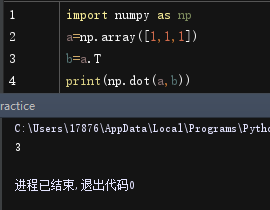
np.dot()函数:
是np中的矩阵乘法，假设 a,b为矩阵，a.dot(b) 等价于 np.dot(a,b)

---

---

第三部分:逻辑回归与神经网络心态( Logistic Regression with a Neural Network mindset

)
你将学会构建学习算法的总体架构，包括:

• 初始化参数
• 计算代价函数及其梯度
• 使用优化算法(梯度下降)
• 按照正确的顺序将上面的三个函数集合到一个主要的模型函数中。

---

3.1 Packages

首先，让我们运行下面的单元格，以导入本次作业中需要的所有包。

• numpy是使用Python进行科学计算的基本包。
• h5py是一个与存储在H5文件中的数据集交互的通用包。
• matplotlib是一个著名的Python绘图库。
• 在这里用PIL和scipy来测试你的模型，在结尾使用你自己的照片。

注意下载版本与自己电脑cpu、操作系统、已安装python版本的适配情况：
版本的含义
Win32 -> 指的就是Windows系统；
64 bit- > 指的是Windows是64位的；
AMD64 -> 指的就是 CPU是x64的；
安装scipy之前先安装numpy-mkl(且二者最好版本相同)

认识一些调用库的语句：

import numpy as np
import matplotlib.pyplot as plt
import h5py
import scipy
from PIL import Image
from scipy import ndimage
from lr_utils import load_dataset
% matplotlib inline

1. lr_utils.py代码如下，你也可以自行打开它查看：
   （需要注意的是，下载好的datasets文件夹放在一个简单的位置，下面语句train_dataset = h5py.File('datasets/train_catvnoncat.h5', “r”)中的datasets/train_catvnoncat.h5应该是你下载好的datasets的绝对路径，然后要保证当前项目中的lr_utils.py是可以成功调用datasets文件夹里的数据集的,因为我是在pycharm上进行复现的，所以Ir_utils.py与主程序同项目，Ir_utils.py通过本地路径访问h5格式的数据集）

import numpy as np
import h5py
def load_dataset():
    train_dataset = h5py.File('datasets/train_catvnoncat.h5', "r")
    train_set_x_orig = np.array(train_dataset["train_set_x"][:]) # your train set features
    train_set_y_orig = np.array(train_dataset["train_set_y"][:]) # your train set labels

    test_dataset = h5py.File('datasets/test_catvnoncat.h5', "r")
    test_set_x_orig = np.array(test_dataset["test_set_x"][:]) # your test set features
    test_set_y_orig = np.array(test_dataset["test_set_y"][:]) # your test set labels

    classes = np.array(test_dataset["list_classes"][:]) # the list of classes
    
    train_set_y_orig = train_set_y_orig.reshape((1, train_set_y_orig.shape[0]))
    test_set_y_orig = test_set_y_orig.reshape((1, test_set_y_orig.shape[0]))
    
    return train_set_x_orig, train_set_y_orig, test_set_x_orig, test_set_y_orig, classes

关于函数load_dataset() 返回的值的含义：

• train_set_x_orig ：保存的是训练集里面的图像数据（本训练集有209张64x64的图像）。
• train_set_y_orig ：保存的是训练集的图像对应的分类值（【0 | 1】，0表示不是猫，1表示是猫）。
• test_set_x_orig ：保存的是测试集里面的图像数据（本训练集有50张64x64的图像）。
• test_set_y_orig ： 保存的是测试集的图像对应的分类值（【0 | 1】，0表示不是猫，1表示是猫）。
• classes ： 保存的是以bytes类型保存的两个字符串数据，数据为：[b’non-cat’ b’cat’]。

2.datasets获取（提取码：2u3w）
3. %matplotlib inline是一个魔法函数（Magic Functions）。官方给出的定义是：IPython有一组预先定义好的所谓的魔法函数（Magic Functions），你可以通过命令行的语法形式来访问它们。
for example：

%matplotlib inline
import matplotlib as mpl
import matplotlib.pyplot as plt
import numpy as np
x = np.linspace(0,10,100)
y_1 = x + 10
plt.plot(x,y_1)
# 但要注意！%matplotlib inline是在jupyter中用的，Pycharm中要把%matplotlib inline改为plt.show()

输出：

---

3.2数据集的准备工作

问题陈述:
给你一个数据集(" data.h5 ")包含:

• 标记为猫(y=1)或非猫(y=0)的m_train图像的训练集

• 标记为猫或非猫的m_test图像测试集

• 每个图像的维度都是(num_px, num_px, 3)，其中3是height=3通道(RGB)。因此，每个图像都是正方形(其中：高度= num_px；宽度= num_px)。

您将构建一个简单的图像识别算法，可以正确地将图片分类为猫或非猫。
让我们更加熟悉数据集。通过运行以下代码加载数据。

# Loading the data (cat/non-cat)
train_set_x_orig, train_set_y, test_set_x_orig, test_set_y, classes = load_dataset()

我们在图像数据集(训练和测试)的末尾添加了**“_orig”**，因为我们要对它们进行预处理。预处理之后，我们将得到train_set_x和test_set_x(标签train_set_y和test_set_y不需要任何预处理)。
train_set_x_orig和test_set_x_orig的每一行都是一个表示图像的数组。您可以通过运行以下代码来可视化一个示例。也可以随意更改索引值并重新运行以查看其他图像。

# Example of a picture
index = 25
plt.imshow(train_set_x_orig[index])
plt.show()
print ("y = " + str(train_set_y[:, index]) + ", it's a '" + classes[np.squeeze(train_set_y[:, index])].decode("utf-8") +  "' picture.")
# 使用np.squeeze的目的是压缩维度，【未压缩】train_set_y[:,index]的值为[1] , 【压缩后】np.squeeze(train_set_y[:,index])的值为1
# 只有压缩后的值才可以进行解码操作
#print("train_set_y=" + str(train_set_y)) #你也可以看一下训练集里面的标签是什么样的。

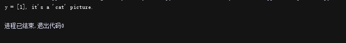
输出：
先有猫片，再输出结论。

y = [1], it's a 'cat' picture.

尝试过程中改过索引值，发现除了index=25，index=2也是猫猫！（总之之前奇怪各种解析博客为啥都是这张黑猫图）

index=2：

验证结论，成立。

index=64

试了试查看index=64在训练集中的标签值，现在暂时看不太懂

同时深度学习中的许多软件错误来自于矩阵/向量维度不适合。如果你能够保持你的矩阵/向量维度是直线的（即秩为1），你便能够有效地消除许多bug。

练习:找到下面的值:

• m_train(训练示例数)

• m_test(测试示例数)

• num_px (= height = width的训练图像)

记住，train_set_x_orig是一个向量数组(m_train, num_px, num_px, 3)。例如，您可以通过编写train_set_x_origin .shape[0]来访问m_train。
代码如下：

### START CODE HERE ### (≈ 3 lines of code)
m_train = train_set_y.shape[1] #训练集里图片的数量。
m_test = test_set_y.shape[1] #测试集里图片的数量。
num_px = train_set_x_orig.shape[1] #训练、测试集里面的图片的宽度和高度（均为64x64）。

#现在看一看我们加载的东西的具体情况
print ("训练集的数量: m_train = " + str(m_train))
print ("测试集的数量 : m_test = " + str(m_test))
print ("每张图片的宽/高 : num_px = " + str(num_px))
print ("每张图片的大小 : (" + str(num_px) + ", " + str(num_px) + ", 3)")
print ("训练集_图片的维数 : " + str(train_set_x_orig.shape))
print ("训练集_标签的维数 : " + str(train_set_y.shape))
print ("测试集_图片的维数: " + str(test_set_x_orig.shape))
print ("测试集_标签的维数: " + str(test_set_y.shape))

输出结果：

训练集的数量: m_train = 209
测试集的数量 : m_test = 50
每张图片的宽/高 : num_px = 64
每张图片的大小 : (64, 64, 3)
训练集_图片的维数 : (209, 64, 64, 3)
训练集_标签的维数 : (1, 209)
测试集_图片的维数: (50, 64, 64, 3)
测试集_标签的维数: (1, 50)

为了方便，您现在应该将数组的维度由(num_px, num_px, 3)规范为（num_px∗num_px∗*∗3,1）。在此之后，我们的训练(和测试)数据集就变成了一个一维的num_array数组，其中每一列代表一个扁平的图像。同时应该具有m_train和m_test列。【每列代表一个平坦的图像】 ，应该有m_train和m_test列。

练习:重新构造训练和测试数据集，使大小(num_px, num_px, 3)的图像被平坦化为一维的单个向量(num_px∗num_px∗ 3,1)

当你想把形状为(a,b,c,d)的矩阵X压平为形状为(b*c*d, a)的矩阵X时，有一个技巧可以使用:

X_flatten = X.reshape(X.shape[0], -1).T      # X.T is the transpose of X

# Reshape the training and test examples

### START CODE HERE ### (≈ 2 lines of code)
train_set_x_flatten = train_set_x_orig.reshape(m_train, -1).T
#将训练集的维度降低并转置。
test_set_x_flatten = test_set_x_orig.reshape(m_test, -1).T
#将测试集的维度降低并转置。

这一段意思是指把数组变为209行的矩阵（因为训练集里有209张图片），但是我懒得算列有多少，于是我就用-1告诉程序你帮我算，最后程序算出来时12288列，我再最后用一个T表示转置，这就变成了12288行，209列(这样每一列都是一张图片的相关信息)。测试集亦如此。

print ("训练集降维最后的维度： " + str(train_set_x_flatten.shape))
print ("训练集_标签的维数 : " + str(train_set_y.shape))
print ("测试集降维之后的维度: " + str(test_set_x_flatten.shape))
print ("测试集_标签的维数 : " + str(test_set_y.shape))
print ("sanity check after reshaping: " + str(train_set_x_flatten[0:5,0]))
#最后一行数组的[0:5,0]表示train_set_x_flatten的两个纬度中：第一个纬度取0-4的元素，第二个纬度取第0行，以逗号作为分隔维度的标识

输出结果：

训练集降维最后的维度： (12288, 209)
训练集_标签的维数 : (1, 209)
测试集降维之后的维度: (12288, 50)
测试集_标签的维数 : (1, 50)
sanity check after reshaping: [17 31 56 22 33]

为了表示彩色图像，必须为每个像素指定红、绿、蓝通道(RGB)，因此像素值实际上是一个由0到255之间的三个数字组成的向量。
机器学习中一个常见的预处理步骤是将数据集集中并标准化，这意味着从每个示例中减去整个numpy数组的均值，然后将每个示例除以整个numpy数组的标准差。但是对于图像数据集，将数据集的每一行除以255(像素通道的最大值)更简单、更方便，而且几乎同样有效。
于是我们试着标准化我们的数据集。

train_set_x = train_set_x_flatten/255.
test_set_x = test_set_x_flatten/255.

你需要记住的是预处理新数据集的常见步骤:

• 找出问题的尺寸和形状(m_train, m_test, num_px，…)
• 重新构造数据集，使每个示例现在都是一维向量(num_px * num_px * 3,1)
• “标准化”处理数据集

以上就是准备数据集的所有理论知识，实际代码如下：

import numpy as np
import matplotlib.pyplot as plt
from lr_utils import load_dataset

def get_data():
    # 将数据加载
    train_set_x_orig, train_set_y, test_set_x_orig, test_set_y, classes = load_dataset()
    # train_set_x_orig 训练集有209张64*64的图像
    # train_set_y 训练集图像对应的标签值[0/1]
    # test_set_x_orig 训练集有50张4*4的图像
    # test_set_y 测试集图像对应的标签值[0/1]
    # classes 保存的是以bytes类型保存的两个字符串数据，数据为[b' non-cat    b' cat']

    # 查看数据
    index = 30
    plt.imshow(train_set_x_orig[index])
    plt.show()
    print("x=" + str(index) + ",y=" + str(train_set_y[:, index]) + ",it's a " + classes[
        np.squeeze(train_set_y[:, index])].decode("UTF-8") + "‘ picture")
    # 使用np.squeeze的目的是压缩维度，【未压缩】train_set_y[:,index]的值为[1] , 【压缩后】np.squeeze(train_set_y[:,index])的值为1
    # 只有压缩后的值才可以进行解码操作
    

    #统计一下数据集中的图片数量
    m_train = train_set_y.shape[1]  # 训练集里图片的数量。
    m_test = test_set_y.shape[1]  # 测试集里图片的数量。
    num_px = train_set_x_orig.shape[1]  # 训练、测试集里面的图片的宽度和高度（均为64x64）。
    print("训练集的数量: m_train = " + str(m_train))
    print("测试集的数量 : m_test = " + str(m_test))
    print("每张图片的宽/高 : num_px = " + str(num_px))
    print("每张图片的大小 : (" + str(num_px) + ", " + str(num_px) + ", 3)")
    print("训练集_图片的维数 : " + str(train_set_x_orig.shape))
    print("训练集_标签的维数 : " + str(train_set_y.shape))
    print("测试集_图片的维数: " + str(test_set_x_orig.shape))
    print("测试集_标签的维数: " + str(test_set_y.shape))
    # a.shape返回的是各维度的长度


    # 处理数据用于神经网络
    train_set_x_flatten = train_set_x_orig.reshape(train_set_x_orig.shape[0], -1).T
    test_set_x_flatten = test_set_x_orig.reshape(test_set_x_orig.shape[0], -1).T
    # 降低维度
    # a.shape[n]返回第n+1维度的长度,此处train_set_x_orig.shape[0]为读取矩阵第一维度的长度，即矩阵行数209，也是样本个数
    # a.reshape(row_size,column_seize)，如代码column_size为-1即不作规定，自动通过行数计算应有的列数
    # 如将（209，64，64，3）的训练集和测试集矩阵，转化为（209，64*64*3）的矩阵，每一行所代表的行向量代表一个图像的64*64像素
    # 而每个像素由红、绿、蓝三种颜色在0~255区间混合而成，故行向量维度为64*64*3
    # 转置
    # 在神经网络中用列向量定义训练样本中的每个样本，并通过行向量方式堆叠会简单许多
    # a.T是a的转置
    # 将（209，64*64*3）的矩阵转置为（64*64*3,209）的矩阵，每一列所代表的列向量代表一个图像的64*64像素，列向量维度为64*64*3
    print("训练集降维最后的维度： " + str(train_set_x_flatten.shape))
    print("训练集_标签的维数 : " + str(train_set_y.shape))
    print("测试集降维之后的维度: " + str(test_set_x_flatten.shape))
    print("测试集_标签的维数 : " + str(test_set_y.shape))
    print("sanity check after reshaping: " + str(train_set_x_flatten[0:5, 0]))
    #最后一行数组的[0:5,0]表示train_set_x_flatten的两个纬度中：第一个纬度取0-4的元素，第二个纬度取第0行，以逗号作为分隔维度的标识


    #标准化我们的数据集
    train_set_x = train_set_x_flatten / 255
    test_set_x = test_set_x_flatten / 255
    # 机器学习中常见的预处理步骤是对数据集进行居中和标准化，便于图片数据集更简单方便的使用
    # 每一行除以255（像素通道的最大值），让标准化数据位于[0，1]之间
    # 由于python的广播机制，直接除以255相当于矩阵中的每个值都除以255

    return train_set_x, train_set_y, test_set_x, test_set_y

---

---

第四部分:学习算法的一般架构

是时候设计一个简单的算法来区分猫的图像和非猫的图像了。
您将使用神经网络思维方式构建逻辑回归。

关键步骤:

• 初始化模型参数

• 通过最小化成本来学习模型参数

• 使用学习到的参数进行预测(在测试集上)

• 分析结果并得出结论

---

---

第五部分:构建神经网络（我们的算法部分）

构建神经网络的主要步骤是:

• 定义模型结构(例如输入特性的数量)

• 初始化模型的参数

• 循环:

  1. 计算实时损耗(正向传播)
  2. 计算当前梯度(反向传播)
  3. 更新参数(梯度下降)

你通常分别构建1-3个，然后将它们集成到一个函数中，我们称之为model()。

---

5.1.辅助函数的使用

练习:使用“Python基础”中的代码，实现sigmoid()。
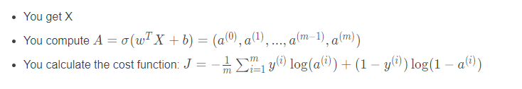
正如你在上面的图中所看到的，你需要计算:
​
进而得到预测值。可以使用np.exp()函数。
代码如下：

# GRADED FUNCTION: sigmoid

def sigmoid(z):
    """
    Compute the sigmoid of z

   参数：
        z  - 任何大小的标量或numpy数组。
    
    返回：
        s  -  sigmoid（z）
    """

    ### START CODE HERE ### (≈ 1 line of code)
    s = 1.0/(1+np.exp(-z))
    ### END CODE HERE ###
    
    return s

实际调用：

print ("sigmoid([0, 2]) = " + str(sigmoid(np.array([0,2]))))

输出结果：

sigmoid([0, 2]) = [ 0.5         0.88079708]

---

5.2.初始化参数

练习:在下面的单元格中实现参数初始化。
你必须把w初始化为一个由0组成的向量。如果不知道要使用哪个numpy函数，请在numpy库的文档中查找np.zeros()。
代码表现：

# GRADED FUNCTION: initialize_with_zeros

def initialize_with_zeros(dim):
    """
    此函数为w创建一个维度为（dim，1）的0向量，并将b初始化为0。
        
        参数：
            dim  - 我们想要的w矢量的大小（或者这种情况下的参数数量）
        
        返回：
            w  - 维度为（dim，1）的初始化向量。
            b  - 初始化的标量（对应于偏差）
    """
    
    ### START CODE HERE ### (≈ 1 line of code)
    w = np.zeros((dim, 1))
    b = 0
    ### END CODE HERE ###
    #使用断言来确保我要的数据是正确的
    #assert的作用是现计算表达式 expression ，如果其值为假（即为0），那么它先向stderr打印一条出错信息，然后通过调用 abort 来终止程序运行。
    assert(w.shape == (dim, 1))#w的维度是(dim,1)
    assert(isinstance(b, float) or isinstance(b, int))
    #isinstance（object，type）的作用：来判断一个对象是否是一个已知的类型。其第一个参数（object）为对象，第二个参数（type）为类型名(int…)或类型名的一个列表((int,list,float)是一个列表)。其返回值为布尔型（True or flase）。

若对象的类型与参数二的类型相同则返回True。若参数二为一个元组，则若对象类型与元组中类型名之一相同即返回True。
    
    return w, b

实际调用：

dim = 2
w, b = initialize_with_zeros(dim)
print ("w = " + str(w))
print ("b = " + str(b))

输出结果：

w = [[ 0.]
 [ 0.]]
b = 0

对于图像输入，w将是维度为(num_px * num_px * 3,1)的数组。

---

5.3.实现一个计算成本函数及其渐变的函数propagate（）

现在已经初始化了参数，您可以执行“向前”和“向后”传播步骤来学习参数。
练习：实现一个propagate()函数，计算代价函数及其梯度。
提示:
向前传播:

这里你可能会用到两种公式：

代码如下：

# GRADED FUNCTION: propagate

def propagate(w, b, X, Y):
    """
    实现前向和后向传播的成本函数及其梯度。
    参数：
        w  - 权重，大小不等的数组（num_px * num_px * 3，1）
        b  - 偏差，一个标量
        X  - 矩阵类型为（num_px * num_px * 3，训练数量）
        Y  - 真正的“标签”矢量（如果非猫则为0，如果是猫则为1），矩阵维度为(1,训练数据数量)

    返回：
        cost- 逻辑回归的负对数似然成本
        dw  - 相对于w的损失梯度，因此与w相同的形状
        db  - 相对于b的损失梯度，因此与b的形状相同
    Tips:
    - Write your code step by step for the propagation. np.log(), np.dot()
    """
    
    m = X.shape[1]
    
    #正向传播
    A = sigmoid(np.dot(w.T, X)+b) 
     #计算激活值，具体可参考上述公式                                   
    cost = -(1.0/m)*np.sum(Y*np.log(A)+(1-Y)*np.log(1-A))
    #计算成本
    
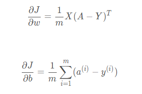
    #反向传播（同样带入公式）
    dw = (1.0/m)*np.dot(X,(A-Y).T)
    db = (1.0/m)*np.sum(A-Y)
    

    #使用断言确保我的数据是正确的
    assert(dw.shape == w.shape)
    assert(db.dtype == float)
    cost = np.squeeze(cost)
    assert(cost.shape == ())
    
    #使用断言确保我的数据是正确的
    grads = {
    
    "dw": dw,
             "db": db}
    
    return grads, cost

实际调用：

w, b, X, Y = np.array([[1.],[2.]]), 2., np.array([[1.,2.,-1.],[3.,4.,-3.2]]), np.array([[1,0,1]])
grads, cost = propagate(w, b, X, Y)
print ("dw = " + str(grads["dw"]))
print ("db = " + str(grads["db"]))
print ("cost = " + str(cost))

输出结果：

dw = [[ 0.99845601]
 [ 2.39507239]]
db = 0.00145557813678
cost = 5.80154531939

---

5.4.优化

• 您已经初始化了参数。
• 你也可以计算代价函数和它的梯度。
• 现在，您需要使用梯度下降来更新参数。

练习:写下优化函数。
目标是通过最小化代价函数J 来学习w 和b。对于参数θ ，更新规则为θ = θ - α *d θ /da，其中α 学习速率。
代码如下：

# GRADED FUNCTION: optimize

def optimize(w, b, X, Y, num_iterations, learning_rate, print_cost = False):
    """
    此函数通过运行梯度下降算法来优化w和b
    参数：
        w  - 权重，大小不等的数组（num_px * num_px * 3，1）
        b  - 偏差，一个标量
        X  - 维度为（num_px * num_px * 3，训练数据的数量）的数组。
        Y  - 真正的“标签”矢量（如果非猫则为0，如果是猫则为1），矩阵维度为(1,训练数据的数量)
        num_iterations  - 优化循环的迭代次数
        learning_rate  - 梯度下降更新规则的学习率
        print_cost  - 每100步打印一次损失值
    
    返回：
        params  - 包含权重w和偏差b的字典
        grads  - 包含权重和偏差相对于成本函数的梯度的字典
        成本 - 优化期间计算的所有成本列表，将用于绘制学习曲线。
    
    提示：
    我们需要写下两个步骤并遍历它们：
        1）计算当前参数的成本和梯度，使用propagate（）。
        2）使用w和b的梯度下降法则更新参数。
    """
    
    costs = []
    
    for i in range(num_iterations):
        
        
        # Cost and gradient calculation (≈ 1-4 lines of code)
        ### START CODE HERE ### 
        grads, cost = propagate(w, b, X, Y)
        ### END CODE HERE ###
        
        # Retrieve derivatives from grads
        dw = grads["dw"]
        db = grads["db"]
        
        # update rule (≈ 2 lines of code)
        ### START CODE HERE ###
        w = w - learning_rate*dw
        b = b - learning_rate*db
        ### END CODE HERE ###
        
        # Record the costs
        if i % 100 == 0:
            costs.append(cost)
        
        # Print the cost every 100 training examples
        if print_cost and i % 100 == 0:
            print ("Cost after iteration %i: %f" %(i, cost))
    
    params = {
    
    "w": w,
              "b": b}
    
    grads = {
    
    "dw": dw,
             "db": db}
    
    return params, grads, costs

实际调用：

params, grads, costs = optimize(w, b, X, Y, num_iterations= 100, learning_rate = 0.009, print_cost = False)

print ("w = " + str(params["w"]))
print ("b = " + str(params["b"]))
print ("dw = " + str(grads["dw"]))
print ("db = " + str(grads["db"]))

输出结果：

w = [[ 0.19033591]
 [ 0.12259159]]
b = 1.92535983008
dw = [[ 0.67752042]
 [ 1.41625495]]
db = 0.219194504541

练习:前面的函数将输出学到的w和b。
我们能够使用w和b预测数据集x的标签。实现predict()函数。计算预测有两个步骤:

• Calculate Yhat = A = σ ( w ^T X + b )
• 将激活函数的结果进行化简：
  • 如果激活值 <= 0.5，a=0
  • 如果激活值 > 0.5，a=1

并将预测存储在向量y_predict中。如果你愿意，你可以在for循环中使用If /else语句(尽管也有一种向量化的方法)。
代码实现：

# GRADED FUNCTION: predict

def predict(w, b, X):
    '''
    使用学习逻辑回归参数logistic （w，b）预测标签是0还是1，
    
    参数：
        w  - 权重，大小不等的数组（num_px * num_px * 3，1）
        b  - 偏差，一个标量
        X  - 维度为（num_px * num_px * 3，训练数据的数量）的数据
    
    返回：
        Y_prediction  - 包含X中所有图片的所有预测【0 | 1】的一个numpy数组（向量）
    
    '''
    
    m = X.shape[1]#图片的数量
    Y_prediction = np.zeros((1,m))
    w = w.reshape(X.shape[0], 1)
    
    #预测猫在图片中出现的概率
    A = sigmoid(np.dot(w.T, X) + b)
    ### END CODE HERE ###
    
    for i in range(A.shape[1]):
        
        # Convert probabilities A[0,i] to actual predictions p[0,i]
        ### START CODE HERE ### (≈ 4 lines of code)
        if A[0,i] > 0.5:
            Y_prediction[0,i] = 1
        else:
            Y_prediction[0,i] = 0
        ### END CODE HERE ###
    
    assert(Y_prediction.shape == (1, m))
    
    return Y_prediction

实际调用：

w = np.array([[0.1124579],[0.23106775]])
b = -0.3
X = np.array([[1.,-1.1,-3.2],[1.2,2.,0.1]])
print ("predictions = " + str(predict(w, b, X)))

输出展示：

predictions = [[ 1.  1.]]

注意:
你已经实现了几个函数的:

• 初始化(w,b)
• 优化损失迭代学习参数(w,b)
• 计算成本和它的梯度-使用梯度下降更新参数
• 使用学习的(w,b)为给定的一组示例预测标签

---

---

第六部分.将所有功能合并到一个模型中

现在您将看到，通过将所有构建块(在前面部分中实现的函数)以正确的顺序组合在一起，整个模型是如何构建的。
练习:实现模型函数。使用下面的符号:

• Y_predict用于测试集中的预测

• Y_prediction_train用于对训练集的预测

• w, cost, optimization()用于输出梯度

代码如下：

# GRADED FUNCTION: model

def model(X_train, Y_train, X_test, Y_test, num_iterations = 2000, learning_rate = 0.5, print_cost = False):
    """
     通过调用之前实现的函数来构建逻辑回归模型
    
    参数：
        X_train  - numpy的数组,维度为（num_px * num_px * 3，m_train）的训练集
        Y_train  - numpy的数组,维度为（1，m_train）（矢量）的训练标签集
        X_test   - numpy的数组,维度为（num_px * num_px * 3，m_test）的测试集
        Y_test   - numpy的数组,维度为（1，m_test）的（向量）的测试标签集
        num_iterations  - 表示用于优化参数的迭代次数的超参数
        learning_rate  - 表示optimize（）更新规则中使用的学习速率的超参数
        print_cost  - 设置为true以每100次迭代打印成本
    
    返回：
        d  - 包含有关模型信息的字典。
    """
  
    w, b = initialize_with_zeros(X_train.shape[0])
    
    parameters, grads, costs = optimize(w, b, X_train, Y_train, num_iterations, learning_rate, print_cost)
    
    #从字典“参数”中检索参数w和b
    w = parameters["w"]
    b = parameters["b"]
    
    #预测测试/训练集的例子
    Y_prediction_test = predict(w, b, X_test)
    Y_prediction_train = predict(w, b, X_train)


    #打印训练后的准确性
    print("train accuracy: {} %".format(100 - np.mean(np.abs(Y_prediction_train - Y_train)) * 100))
    print("test accuracy: {} %".format(100 - np.mean(np.abs(Y_prediction_test - Y_test)) * 100))

    
    d = {
    
    "costs": costs,
         "Y_prediction_test": Y_prediction_test, 
         "Y_prediction_train" : Y_prediction_train, 
         "w" : w, 
         "b" : b,
         "learning_rate" : learning_rate,
         "num_iterations": num_iterations}
    
    return d

运行以下单元格来训练模型：

d = model(train_set_x, train_set_y, test_set_x, test_set_y, num_iterations = 2000, learning_rate = 0.005, print_cost = True)

输出结果：

Cost after iteration 0: 0.693147
Cost after iteration 100: 0.584508
Cost after iteration 200: 0.466949
Cost after iteration 300: 0.376007
Cost after iteration 400: 0.331463
Cost after iteration 500: 0.303273
Cost after iteration 600: 0.279880
Cost after iteration 700: 0.260042
Cost after iteration 800: 0.242941
Cost after iteration 900: 0.228004
Cost after iteration 1000: 0.214820
Cost after iteration 1100: 0.203078
Cost after iteration 1200: 0.192544
Cost after iteration 1300: 0.183033
Cost after iteration 1400: 0.174399
Cost after iteration 1500: 0.166521
Cost after iteration 1600: 0.159305
Cost after iteration 1700: 0.152667
Cost after iteration 1800: 0.146542
Cost after iteration 1900: 0.140872
train accuracy: 99.04306220095694 %
test accuracy: 70.0 %

点评:
训练准确率接近100%说明这是一个很好的检查:您的模型正在工作，并且有足够的容量来拟合训练数据。测试误差为68%。对于这个简单的模型来说，它实际上并不坏，因为我们使用的数据集很小，而且逻辑回归是一个线性分类器。但不用担心，下周你会建立一个更好的分类器!
此外，您还可以看到模型明显对训练数据进行过拟合。在本专门化的后面，您将学习如何减少过拟合，例如使用正则化。使用下面的代码(并更改索引变量)，您可以查看测试集图片上的预测。

我们再画一下代价函数和梯度。

#绘制图
costs = np.squeeze(d['costs'])
plt.plot(costs)
plt.ylabel('cost')
plt.xlabel('iterations (per hundreds)')
plt.title("Learning rate =" + str(d["learning_rate"]))
plt.show()

跑一波出来的效果图是这样的，可以看到成本下降，它显示参数正在被学习：

解释:
可以看到成本在下降。这表明参数正在被学习。然而，您可以看到您可以在训练集中对模型进行更多的训练。尝试增加上面单元中的迭代次数并重新运行单元。你可能会看到训练集的精度上升了，但是测试集的精度下降了。这叫做过拟合。

---

---

第七部分.学习速率的选择

祝贺您构建了您的第一个图像分类模型。让我们进一步分析它，并检查学习速率α的可能选择。
提示:
为了让梯度下降起作用，你必须明智地选择学习速率。学习速率α决定了我们更新参数的速度。如果学习率过大，我们可能会“超调”最优值。同样，如果它太小，我们将需要多次迭代才能收敛到最佳值。这就是为什么使用一个调整好的学习速率是至关重要的。
让我们将模型的学习曲线与几种学习率的选择进行比较。运行下面的单元格。大概需要1分钟。也可以尝试不同的值，而不是我们初始化learning_rates变量所包含的三个值，看看会发生什么。

learning_rates = [0.01, 0.001, 0.0001]
models = {
    
    }
for i in learning_rates:
    print ("learning rate is: " + str(i))
    models[str(i)] = model(train_set_x, train_set_y, test_set_x, test_set_y, num_iterations = 1500, learning_rate = i, print_cost = False)
    print ('\n' + "-------------------------------------------------------" + '\n')

for i in learning_rates:
    plt.plot(np.squeeze(models[str(i)]["costs"]), label= str(models[str(i)]["learning_rate"]))

plt.ylabel('cost')
plt.xlabel('iterations')

legend = plt.legend(loc='upper center', shadow=True)
frame = legend.get_frame()
frame.set_facecolor('0.90')
plt.show()

运行结果是：

learning rate is: 0.01
train accuracy: 99.52153110047847 %
test accuracy: 68.0 %

-------------------------------------------------------

learning rate is: 0.001
train accuracy: 88.99521531100478 %
test accuracy: 64.0 %

-------------------------------------------------------

learning rate is: 0.0001
train accuracy: 68.42105263157895 %
test accuracy: 36.0 %

-------------------------------------------------------

解释:

• 不同的学习速率会产生不同的代价，从而产生不同的预测结果。
• 如果学习率太大(0.01)，代价可能会上下振荡。它甚至可能会发散(尽管在这个例子中，使用0.01最终仍然会得到一个较好的成本值)。
• 更低的成本并不意味着更好的模式。你必须检查是否存在过拟合。当训练准确率远远高于测试准确率时就会出现这种情况。
• 在深度学习方面，我们通常建议您:
  • 选择能更好地使代价函数最小化的学习率。
  • 如果你的模型过拟合，使用其他技术来减少过拟合。(我们将在以后的视频中讨论这个。)

---

---

第八部分. 用自己的图像测试

恭喜你完成了这项任务。您可以使用自己的图像并查看模型的输出。这样做:

1. 点击这个笔记本上栏的“文件”，然后点击“打开”去你的Coursera中心。
2. 将您的图像添加到这个Jupyter Notebook的“图像”文件夹中
3. 在下面的代码中更改图片的名称
4. 运行代码并检查算法是否正确(1 = cat, 0 = non-cat)!

而以下代码是在pycharm（同时配合anaconda搭建的虚拟环境）实现的，因为pycharm本身下载packages提到的scipy库时总是版本不适配：

代码表现：

print("====================测试model====================")
d = model(train_set_x, train_set_y, test_set_x, test_set_y, num_iterations = 2000, learning_rate = 0.005, print_cost = True)

## START CODE HERE ## (PUT YOUR IMAGE NAME)
my_image = "cat.jpg"   # change this to the name of your image file
my_label_y=[1]# the true class of your image (1 -> cat, 0 -> non-cat)
## END CODE HERE ##

# We preprocess the image to fit your algorithm.
fname = "D:/" + my_image
image = np.array(matplotlib.pyplot.imread(fname))
# my_image = scipy.misc.imresize(image, size=(num_px,num_px)).reshape((1, num_px*num_px*3)).T
my_image = np.array(Image.fromarray(image).resize(size=(num_px,num_px))).reshape((1, num_px*num_px*3)).T
my_predicted_image = predict(d["w"], d["b"], my_image)


plt.imshow(image)
print("y = " + str(np.squeeze(my_predicted_image)) + ", your algorithm predicts a \"" + classes[int(np.squeeze(my_predicted_image)),].decode("utf-8") +  "\" picture.")

输出：

再换个不是猫猫的图片识别：

识别成功！猫猫，姐姐爱你！

注意：

1. 预处理数据集很重要
2. 您分别实现了每个函数:initialize()、propagate()、optimize()。然后构建了一个model()
3. 3.调整学习速率(这是“超参数”的一个例子)可以对算法产生很大的影响。在本课程后面你会看到更多的例子!

---

---

第九部分. 完整代码

下列代码是上文用于测试学习速率的完整代码：

import numpy as np
import matplotlib.pyplot as plt
import h5py
from lr_utils import load_dataset

train_set_x_orig , train_set_y , test_set_x_orig , test_set_y , classes = load_dataset()

m_train = train_set_y.shape[1] #训练集里图片的数量。
m_test = test_set_y.shape[1] #测试集里图片的数量。
num_px = train_set_x_orig.shape[1] #训练、测试集里面的图片的宽度和高度（均为64x64）。

#现在看一看我们加载的东西的具体情况
print ("训练集的数量: m_train = " + str(m_train))
print ("测试集的数量 : m_test = " + str(m_test))
print ("每张图片的宽/高 : num_px = " + str(num_px))
print ("每张图片的大小 : (" + str(num_px) + ", " + str(num_px) + ", 3)")
print ("训练集_图片的维数 : " + str(train_set_x_orig.shape))
print ("训练集_标签的维数 : " + str(train_set_y.shape))
print ("测试集_图片的维数: " + str(test_set_x_orig.shape))
print ("测试集_标签的维数: " + str(test_set_y.shape))

#将训练集的维度降低并转置。
train_set_x_flatten  = train_set_x_orig.reshape(train_set_x_orig.shape[0],-1).T
#将测试集的维度降低并转置。
test_set_x_flatten = test_set_x_orig.reshape(test_set_x_orig.shape[0], -1).T

print ("训练集降维最后的维度： " + str(train_set_x_flatten.shape))
print ("训练集_标签的维数 : " + str(train_set_y.shape))
print ("测试集降维之后的维度: " + str(test_set_x_flatten.shape))
print ("测试集_标签的维数 : " + str(test_set_y.shape))

train_set_x = train_set_x_flatten / 255
test_set_x = test_set_x_flatten / 255

def sigmoid(z):
    """
    Compute the sigmoid of z

   参数：
        z  - 任何大小的标量或numpy数组。

    返回：
        s  -  sigmoid（z）
    """

    ### START CODE HERE ### (≈ 1 line of code)
    s = 1.0 / (1 + np.exp(-z))
    ### END CODE HERE ###

    return s
def initialize_with_zeros(dim):
    """
    此函数为w创建一个维度为（dim，1）的0向量，并将b初始化为0。

        参数：
            dim  - 我们想要的w矢量的大小（或者这种情况下的参数数量）

        返回：
            w  - 维度为（dim，1）的初始化向量。
            b  - 初始化的标量（对应于偏差）
    """

    ### START CODE HERE ### (≈ 1 line of code)
    w = np.zeros((dim, 1))
    b = 0
    ### END CODE HERE ###
    # 使用断言来确保我要的数据是正确的
    # assert的作用是现计算表达式 expression ，如果其值为假（即为0），那么它先向stderr打印一条出错信息，然后通过调用 abort 来终止程序运行。
    assert (w.shape == (dim, 1))  # w的维度是(dim,1)
    assert (isinstance(b, float) or isinstance(b, int))
    # isinstance（object，type）的作用：来判断一个对象是否是一个已知的类型。其第一个参数（object）为对象，第二个参数（type）为类型名(int…)或类型名的一个列表((int,list,float)是一个列表)。其返回值为布尔型（True or flase）。
    #若对象的类型与参数二的类型相同则返回True。若参数二为一个元组，则若对象类型与元组中类型名之一相同即返回True。
    return w, b
def propagate(w, b, X, Y):
    """
    实现前向和后向传播的成本函数及其梯度。
    参数：
        w  - 权重，大小不等的数组（num_px * num_px * 3，1）
        b  - 偏差，一个标量
        X  - 矩阵类型为（num_px * num_px * 3，训练数量）
        Y  - 真正的“标签”矢量（如果非猫则为0，如果是猫则为1），矩阵维度为(1,训练数据数量)

    返回：
        cost- 逻辑回归的负对数似然成本
        dw  - 相对于w的损失梯度，因此与w相同的形状
        db  - 相对于b的损失梯度，因此与b的形状相同
    Tips:
    - Write your code step by step for the propagation. np.log(), np.dot()
    """

    m = X.shape[1]

    # 正向传播
    A = sigmoid(np.dot(w.T, X) + b)
    # 计算激活值，具体可参考上述公式
    cost = -(1.0 / m) * np.sum(Y * np.log(A) + (1 - Y) * np.log(1 - A))
    # 计算成本

    # 反向传播（同样带入公式）
    dw = (1.0 / m) * np.dot(X, (A - Y).T)
    db = (1.0 / m) * np.sum(A - Y)

    # 使用断言确保我的数据是正确的
    assert (dw.shape == w.shape)
    assert (db.dtype == float)
    cost = np.squeeze(cost)
    assert (cost.shape == ())

    # 使用断言确保我的数据是正确的
    grads = {
    
    "dw": dw,
             "db": db}

    return grads, cost
def optimize(w, b, X, Y, num_iterations, learning_rate, print_cost=False):
    """
    此函数通过运行梯度下降算法来优化w和b
    参数：
        w  - 权重，大小不等的数组（num_px * num_px * 3，1）
        b  - 偏差，一个标量
        X  - 维度为（num_px * num_px * 3，训练数据的数量）的数组。
        Y  - 真正的“标签”矢量（如果非猫则为0，如果是猫则为1），矩阵维度为(1,训练数据的数量)
        num_iterations  - 优化循环的迭代次数
        learning_rate  - 梯度下降更新规则的学习率
        print_cost  - 每100步打印一次损失值

    返回：
        params  - 包含权重w和偏差b的字典
        grads  - 包含权重和偏差相对于成本函数的梯度的字典
        成本 - 优化期间计算的所有成本列表，将用于绘制学习曲线。

    提示：
    我们需要写下两个步骤并遍历它们：
        1）计算当前参数的成本和梯度，使用propagate（）。
        2）使用w和b的梯度下降法则更新参数。
    """

    costs = []

    for i in range(num_iterations):

        # Cost and gradient calculation (≈ 1-4 lines of code)
        ### START CODE HERE ###
        grads, cost = propagate(w, b, X, Y)
        ### END CODE HERE ###

        # Retrieve derivatives from grads
        dw = grads["dw"]
        db = grads["db"]

        # update rule (≈ 2 lines of code)
        ### START CODE HERE ###
        w = w - learning_rate * dw
        b = b - learning_rate * db
        ### END CODE HERE ###

        # Record the costs
        if i % 100 == 0:
            costs.append(cost)

        # Print the cost every 100 training examples
        if print_cost and i % 100 == 0:
            print("Cost after iteration %i: %f" % (i, cost))

    params = {
    
    "w": w,
              "b": b}

    grads = {
    
    "dw": dw,
             "db": db}

    return params, grads, costs
def predict(w, b, X):
    '''
    使用学习逻辑回归参数logistic （w，b）预测标签是0还是1，

    参数：
        w  - 权重，大小不等的数组（num_px * num_px * 3，1）
        b  - 偏差，一个标量
        X  - 维度为（num_px * num_px * 3，训练数据的数量）的数据

    返回：
        Y_prediction  - 包含X中所有图片的所有预测【0 | 1】的一个numpy数组（向量）

    '''

    m = X.shape[1]  # 图片的数量
    Y_prediction = np.zeros((1, m))
    w = w.reshape(X.shape[0], 1)

    # 预测猫在图片中出现的概率
    A = sigmoid(np.dot(w.T, X) + b)
    ### END CODE HERE ###

    for i in range(A.shape[1]):

        # Convert probabilities A[0,i] to actual predictions p[0,i]
        ### START CODE HERE ### (≈ 4 lines of code)
        if A[0, i] > 0.5:
            Y_prediction[0, i] = 1
        else:
            Y_prediction[0, i] = 0
            ### END CODE HERE ###

    assert (Y_prediction.shape == (1, m))

    return Y_prediction
def model(X_train, Y_train, X_test, Y_test, num_iterations=2000, learning_rate=0.5, print_cost=False):
    """
     通过调用之前实现的函数来构建逻辑回归模型

    参数：
        X_train  - numpy的数组,维度为（num_px * num_px * 3，m_train）的训练集
        Y_train  - numpy的数组,维度为（1，m_train）（矢量）的训练标签集
        X_test   - numpy的数组,维度为（num_px * num_px * 3，m_test）的测试集
        Y_test   - numpy的数组,维度为（1，m_test）的（向量）的测试标签集
        num_iterations  - 表示用于优化参数的迭代次数的超参数
        learning_rate  - 表示optimize（）更新规则中使用的学习速率的超参数
        print_cost  - 设置为true以每100次迭代打印成本

    返回：
        d  - 包含有关模型信息的字典。
    """

    w, b = initialize_with_zeros(X_train.shape[0])

    parameters, grads, costs = optimize(w, b, X_train, Y_train, num_iterations, learning_rate, print_cost)

    # 从字典“参数”中检索参数w和b
    w = parameters["w"]
    b = parameters["b"]

    # 预测测试/训练集的例子
    Y_prediction_test = predict(w, b, X_test)
    Y_prediction_train = predict(w, b, X_train)

    # 打印训练后的准确性
    print("train accuracy: {} %".format(100 - np.mean(np.abs(Y_prediction_train - Y_train)) * 100))
    print("test accuracy: {} %".format(100 - np.mean(np.abs(Y_prediction_test - Y_test)) * 100))

    d = {
    
    "costs": costs,
         "Y_prediction_test": Y_prediction_test,
         "Y_prediction_train": Y_prediction_train,
         "w": w,
         "b": b,
         "learning_rate": learning_rate,
         "num_iterations": num_iterations}

    return d
print("====================测试model====================")
learning_rates = [0.01, 0.001, 0.0001]
models = {
    
    }
for i in learning_rates:
    print ("learning rate is: " + str(i))
    models[str(i)] = model(train_set_x, train_set_y, test_set_x, test_set_y, num_iterations = 1500, learning_rate = i, print_cost = False)
    print ('\n' + "-------------------------------------------------------" + '\n')

for i in learning_rates:
    plt.plot(np.squeeze(models[str(i)]["costs"]), label= str(models[str(i)]["learning_rate"]))

plt.ylabel('cost')
plt.xlabel('iterations')

legend = plt.legend(loc='upper center', shadow=True)
frame = legend.get_frame()
frame.set_facecolor('0.90')
plt.show()

适配自己的图片识别的的代码如下（注意开头要加上：import matplotlib）：

import numpy as np
import matplotlib
import matplotlib.pyplot as plt
import h5py
import scipy
from PIL import Image
from scipy import ndimage
from lr_utils import load_dataset

train_set_x_orig , train_set_y , test_set_x_orig , test_set_y , classes = load_dataset()

m_train = train_set_y.shape[1] #训练集里图片的数量。
m_test = test_set_y.shape[1] #测试集里图片的数量。
num_px = train_set_x_orig.shape[1] #训练、测试集里面的图片的宽度和高度（均为64x64）。

#现在看一看我们加载的东西的具体情况
print ("训练集的数量: m_train = " + str(m_train))
print ("测试集的数量 : m_test = " + str(m_test))
print ("每张图片的宽/高 : num_px = " + str(num_px))
print ("每张图片的大小 : (" + str(num_px) + ", " + str(num_px) + ", 3)")
print ("训练集_图片的维数 : " + str(train_set_x_orig.shape))
print ("训练集_标签的维数 : " + str(train_set_y.shape))
print ("测试集_图片的维数: " + str(test_set_x_orig.shape))
print ("测试集_标签的维数: " + str(test_set_y.shape))

#将训练集的维度降低并转置。
train_set_x_flatten  = train_set_x_orig.reshape(train_set_x_orig.shape[0],-1).T
#将测试集的维度降低并转置。
test_set_x_flatten = test_set_x_orig.reshape(test_set_x_orig.shape[0], -1).T

print ("训练集降维最后的维度： " + str(train_set_x_flatten.shape))
print ("训练集_标签的维数 : " + str(train_set_y.shape))
print ("测试集降维之后的维度: " + str(test_set_x_flatten.shape))
print ("测试集_标签的维数 : " + str(test_set_y.shape))

train_set_x = train_set_x_flatten / 255
test_set_x = test_set_x_flatten / 255

def sigmoid(z):
    """
    Compute the sigmoid of z

   参数：
        z  - 任何大小的标量或numpy数组。

    返回：
        s  -  sigmoid（z）
    """

    ### START CODE HERE ### (≈ 1 line of code)
    s = 1.0 / (1 + np.exp(-z))
    ### END CODE HERE ###

    return s
def initialize_with_zeros(dim):
    """
    此函数为w创建一个维度为（dim，1）的0向量，并将b初始化为0。

        参数：
            dim  - 我们想要的w矢量的大小（或者这种情况下的参数数量）

        返回：
            w  - 维度为（dim，1）的初始化向量。
            b  - 初始化的标量（对应于偏差）
    """

    ### START CODE HERE ### (≈ 1 line of code)
    w = np.zeros((dim, 1))
    b = 0
    ### END CODE HERE ###
    # 使用断言来确保我要的数据是正确的
    # assert的作用是现计算表达式 expression ，如果其值为假（即为0），那么它先向stderr打印一条出错信息，然后通过调用 abort 来终止程序运行。
    assert (w.shape == (dim, 1))  # w的维度是(dim,1)
    assert (isinstance(b, float) or isinstance(b, int))
    # isinstance（object，type）的作用：来判断一个对象是否是一个已知的类型。其第一个参数（object）为对象，第二个参数（type）为类型名(int…)或类型名的一个列表((int,list,float)是一个列表)。其返回值为布尔型（True or flase）。
    #若对象的类型与参数二的类型相同则返回True。若参数二为一个元组，则若对象类型与元组中类型名之一相同即返回True。
    return w, b
def propagate(w, b, X, Y):
    """
    实现前向和后向传播的成本函数及其梯度。
    参数：
        w  - 权重，大小不等的数组（num_px * num_px * 3，1）
        b  - 偏差，一个标量
        X  - 矩阵类型为（num_px * num_px * 3，训练数量）
        Y  - 真正的“标签”矢量（如果非猫则为0，如果是猫则为1），矩阵维度为(1,训练数据数量)

    返回：
        cost- 逻辑回归的负对数似然成本
        dw  - 相对于w的损失梯度，因此与w相同的形状
        db  - 相对于b的损失梯度，因此与b的形状相同
    Tips:
    - Write your code step by step for the propagation. np.log(), np.dot()
    """

    m = X.shape[1]

    # 正向传播
    A = sigmoid(np.dot(w.T, X) + b)
    # 计算激活值，具体可参考上述公式
    cost = -(1.0 / m) * np.sum(Y * np.log(A) + (1 - Y) * np.log(1 - A))
    # 计算成本

    # 反向传播（同样带入公式）
    dw = (1.0 / m) * np.dot(X, (A - Y).T)
    db = (1.0 / m) * np.sum(A - Y)

    # 使用断言确保我的数据是正确的
    assert (dw.shape == w.shape)
    assert (db.dtype == float)
    cost = np.squeeze(cost)
    assert (cost.shape == ())

    # 使用断言确保我的数据是正确的
    grads = {
    
    "dw": dw,
             "db": db}

    return grads, cost
def optimize(w, b, X, Y, num_iterations, learning_rate, print_cost=False):
    """
    此函数通过运行梯度下降算法来优化w和b
    参数：
        w  - 权重，大小不等的数组（num_px * num_px * 3，1）
        b  - 偏差，一个标量
        X  - 维度为（num_px * num_px * 3，训练数据的数量）的数组。
        Y  - 真正的“标签”矢量（如果非猫则为0，如果是猫则为1），矩阵维度为(1,训练数据的数量)
        num_iterations  - 优化循环的迭代次数
        learning_rate  - 梯度下降更新规则的学习率
        print_cost  - 每100步打印一次损失值

    返回：
        params  - 包含权重w和偏差b的字典
        grads  - 包含权重和偏差相对于成本函数的梯度的字典
        成本 - 优化期间计算的所有成本列表，将用于绘制学习曲线。

    提示：
    我们需要写下两个步骤并遍历它们：
        1）计算当前参数的成本和梯度，使用propagate（）。
        2）使用w和b的梯度下降法则更新参数。
    """

    costs = []

    for i in range(num_iterations):

        # Cost and gradient calculation (≈ 1-4 lines of code)
        ### START CODE HERE ###
        grads, cost = propagate(w, b, X, Y)
        ### END CODE HERE ###

        # Retrieve derivatives from grads
        dw = grads["dw"]
        db = grads["db"]

        # update rule (≈ 2 lines of code)
        ### START CODE HERE ###
        w = w - learning_rate * dw
        b = b - learning_rate * db
        ### END CODE HERE ###

        # Record the costs
        if i % 100 == 0:
            costs.append(cost)

        # Print the cost every 100 training examples
        if print_cost and i % 100 == 0:
            print("Cost after iteration %i: %f" % (i, cost))

    params = {
    
    "w": w,
              "b": b}

    grads = {
    
    "dw": dw,
             "db": db}

    return params, grads, costs
def predict(w, b, X):
    '''
    使用学习逻辑回归参数logistic （w，b）预测标签是0还是1，

    参数：
        w  - 权重，大小不等的数组（num_px * num_px * 3，1）
        b  - 偏差，一个标量
        X  - 维度为（num_px * num_px * 3，训练数据的数量）的数据

    返回：
        Y_prediction  - 包含X中所有图片的所有预测【0 | 1】的一个numpy数组（向量）

    '''

    m = X.shape[1]  # 图片的数量
    Y_prediction = np.zeros((1, m))
    w = w.reshape(X.shape[0], 1)

    # 预测猫在图片中出现的概率
    A = sigmoid(np.dot(w.T, X) + b)
    ### END CODE HERE ###

    for i in range(A.shape[1]):

        # Convert probabilities A[0,i] to actual predictions p[0,i]
        ### START CODE HERE ### (≈ 4 lines of code)
        if A[0, i] > 0.5:
            Y_prediction[0, i] = 1
        else:
            Y_prediction[0, i] = 0
            ### END CODE HERE ###

    assert (Y_prediction.shape == (1, m))

    return Y_prediction
def model(X_train, Y_train, X_test, Y_test, num_iterations=2000, learning_rate=0.5, print_cost=False):
    """
     通过调用之前实现的函数来构建逻辑回归模型

    参数：
        X_train  - numpy的数组,维度为（num_px * num_px * 3，m_train）的训练集
        Y_train  - numpy的数组,维度为（1，m_train）（矢量）的训练标签集
        X_test   - numpy的数组,维度为（num_px * num_px * 3，m_test）的测试集
        Y_test   - numpy的数组,维度为（1，m_test）的（向量）的测试标签集
        num_iterations  - 表示用于优化参数的迭代次数的超参数
        learning_rate  - 表示optimize（）更新规则中使用的学习速率的超参数
        print_cost  - 设置为true以每100次迭代打印成本

    返回：
        d  - 包含有关模型信息的字典。
    """

    w, b = initialize_with_zeros(X_train.shape[0])

    parameters, grads, costs = optimize(w, b, X_train, Y_train, num_iterations, learning_rate, print_cost)

    # 从字典“参数”中检索参数w和b
    w = parameters["w"]
    b = parameters["b"]

    # 预测测试/训练集的例子
    Y_prediction_test = predict(w, b, X_test)
    Y_prediction_train = predict(w, b, X_train)

    # 打印训练后的准确性
    print("train accuracy: {} %".format(100 - np.mean(np.abs(Y_prediction_train - Y_train)) * 100))
    print("test accuracy: {} %".format(100 - np.mean(np.abs(Y_prediction_test - Y_test)) * 100))

    d = {
    
    "costs": costs,
         "Y_prediction_test": Y_prediction_test,
         "Y_prediction_train": Y_prediction_train,
         "w": w,
         "b": b,
         "learning_rate": learning_rate,
         "num_iterations": num_iterations}

    return d
print("====================测试model====================")
d = model(train_set_x, train_set_y, test_set_x, test_set_y, num_iterations = 2000, learning_rate = 0.005, print_cost = True)

## START CODE HERE ## (PUT YOUR IMAGE NAME)
my_image = "dog.jpg"   # change this to the name of your image file
my_label_y=[1]# the true class of your image (1 -> cat, 0 -> non-cat)
## END CODE HERE ##

# We preprocess the image to fit your algorithm.
fname = "D:/" + my_image
image = np.array(matplotlib.pyplot.imread(fname))
# my_image = scipy.misc.imresize(image, size=(num_px,num_px)).reshape((1, num_px*num_px*3)).T
my_image = np.array(Image.fromarray(image).resize(size=(num_px,num_px))).reshape((1, num_px*num_px*3)).T
my_predicted_image = predict(d["w"], d["b"], my_image)


plt.imshow(image)
print("y = " + str(np.squeeze(my_predicted_image)) + ", your algorithm predicts a \"" + classes[int(np.squeeze(my_predicted_image)),].decode("utf-8") +  "\" picture.")