前言

这篇博客主要记录"吴恩达depplearning系列课程"第三周编程作业代码+自己的补充理解的相关内容，以作为学习记录。学习过程中借鉴了各位大佬的代码，想要追根溯源的朋友可以看这几位大佬的博客：大树先生的博客(英文版)，何宽（中文版）
作为初学者，本文的代码是自己当前能做到的”终极满意缝合怪“，同时部分原搬的代码也加了很多注释，便于理解。

numpy是使用Python进行科学计算的基本包。
sklearn为数据挖掘和数据分析提供了简单高效的工具。
matplotlib是一个用Python绘制图形的库。
testCases_v2提供了一些测试示例来评估函数的正确性（该文件放于文末第六部分）
planar_utils提供了用于此赋值的各种有用函数（该文件内容放于文末第七部分）

import numpy as np
import matplotlib.pyplot as plt
from testCases import *
import sklearn
import sklearn.datasets
import sklearn.linear_model
from planar_utils import plot_decision_boundary, sigmoid, load_planar_dataset, load_extra_datasets

np.random.seed(1) #设置一个固定的随机种子，以保证接下来的步骤中我们的结果是一致的。

第2部分:加载和查看数据集

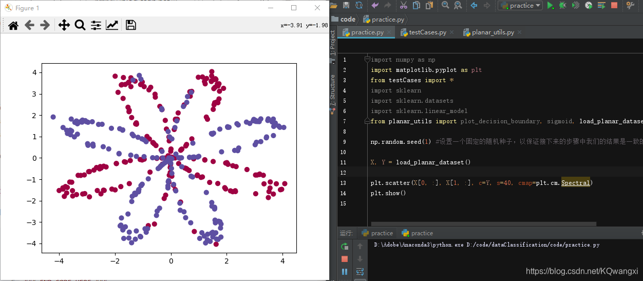
首先，我们来看看我们将要使用的数据集，下面的代码会将一个花的图案的2类数据集加载到变量X和Y中。

X, Y = load_planar_dataset()
plt.scatter(X[0, :], X[1, :], c=Y, s=40, cmap=plt.cm.Spectral) #绘制散点图

# 上一语句如出现问题，请使用下面的语句：
plt.scatter(X[0, :], X[1, :], c=np.squeeze(Y), s=40, cmap=plt.cm.Spectral) #绘制散点图

在这里插入图片描述

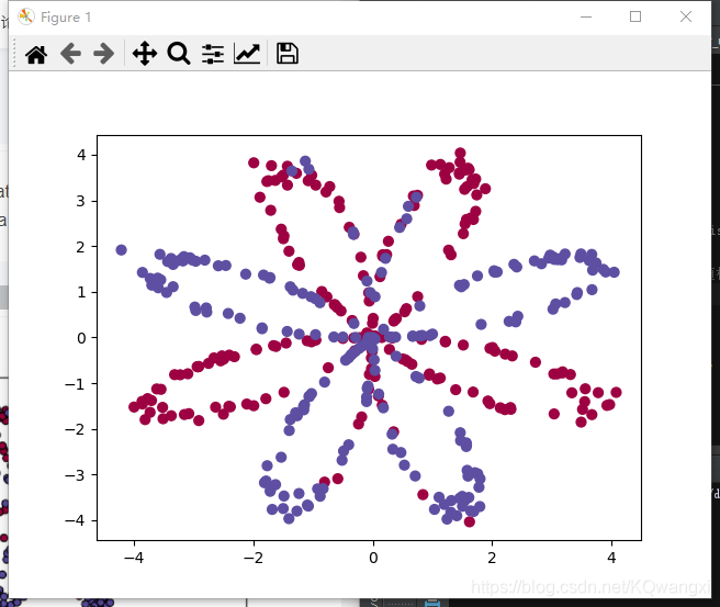
使用matplotlib可视化数据集。数据看起来像一朵“花”，有一些红色（标签y=0）和一些蓝色（y=1）点。你的目标是建立一个模型来适应这些数据。
在这里插入图片描述

我们现在有：

包含特征的numpy数组（矩阵）X（x1，x2）
包含标签的numpy数组（向量）(红色：0, 蓝色：1).

首先让我们更好地了解我们的数据是什么样的。
练习：你有多少个训练例子？另外，变量X和Y的形状是什么？
提示：如何获得numpy数组的形状？

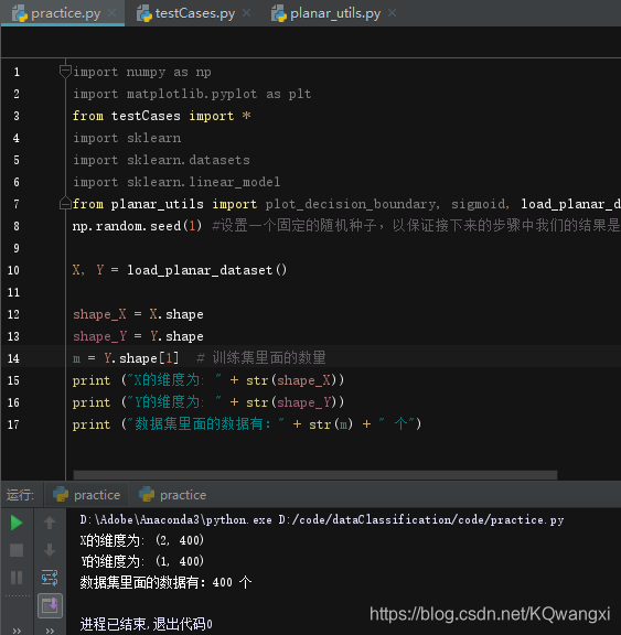
shape_X = X.shape
shape_Y = Y.shape
m = Y.shape[1]  # 训练集里面的数量

print ("X的维度为: " + str(shape_X))
print ("Y的维度为: " + str(shape_Y))
print ("数据集里面的数据有：" + str(m) + " 个")

运行结果为：

X的维度为: (2, 400)
Y的维度为: (1, 400)
数据集里面的数据有：400 个

在这里插入图片描述

第3部分:查看简单的Logistic回归的分类效果

在建立一个完整的神经网络之前，让我们先看看logistic回归如何处理这个问题。您可以使用sklearn的内置函数来实现这一点。运行下面的代码在数据集上训练logistic回归分类器。

扫描二维码关注公众号，回复： 12926817 查看本文章

#训练logistic回归分类器
clf = sklearn.linear_model.LogisticRegressionCV()
clf.fit(X.T,Y.T)

然后发现打印如下信息：

C:\Users\17876\AppData\Roaming\Python\Python38\site-packages\sklearn\utils\validation.py:63: DataConversionWarning: A column-vector y was passed when a 1d array was expected. Please change the shape of y to (n_samples, ), for example using ravel().
  return f(*args, **kwargs)

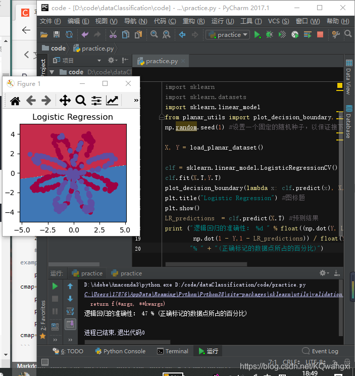
现在可以绘制这些模型的决策边界。运行下面的代码。

plot_decision_boundary(lambda x: clf.predict(x), X, Y) #绘制决策边界
plt.title("Logistic Regression") #图标题
LR_predictions  = clf.predict(X.T) #预测结果
print ("逻辑回归的准确性： %d " % float((np.dot(Y, LR_predictions) + 
		np.dot(1 - Y,1 - LR_predictions)) / float(Y.size) * 100) +
       "% " + "(正确标记的数据点所占的百分比)")

打印内容：

逻辑回归的准确性： 47 % (正确标记的数据点所占的百分比)

就像这样：
在这里插入图片描述
这一步修改代码为：

clf = sklearn.linear_model.LogisticRegressionCV()
clf.fit(X.T,Y.T)
plot_decision_boundary(lambda x: predict(parameters,x.T), X, np.squeeze(Y)) #绘制决策边界
plt.title("Decision Boundary for hidden layer size " + str(4))
LR_predictions  = clf.predict(X.T) #预测结果
print ("逻辑回归的准确性： %d " % float((np.dot(Y, LR_predictions) +
		np.dot(1 - Y,1 - LR_predictions)) / float(Y.size) * 100) +
       "% " + "(正确标记的数据点所占的百分比)")
plt.show()

在这里插入图片描述

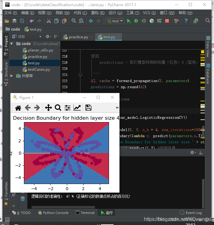
准确性只有47%的原因是数据集不是线性可分的，所以逻辑回归表现不佳，现在我们正式开始构建神经网络
plot_decision_boundary:

def plot_decision_boundary(model, X, y):
    # 设置最大值和最小值，并给它们填充变量
    x_min, x_max = X[0, :].min() - 1, X[0, :].max() + 1
    y_min, y_max = X[1, :].min() - 1, X[1, :].max() + 1
    h = 0.01
    # 生成一个点的网格，它们之间的距离为h
    xx, yy = np.meshgrid(np.arange(x_min, x_max, h), np.arange(y_min, y_max, h))
    # 预测整个网格的函数值
    Z = model(np.c_[xx.ravel(), yy.ravel()])
    Z = Z.reshape(xx.shape)
    # 绘制等高线和训练示例
    plt.contourf(xx, yy, Z, cmap=plt.cm.Spectral)
    plt.ylabel('x2')
    plt.xlabel('x1')
    plt.scatter(X[0, :], X[1, :], c=y, cmap=plt.cm.Spectral)

第四部分:搭建神经网络

Logistic回归在“花数据集”上效果不佳。我们要训练一个只有一个隐藏层的神经网络。
模型如下：
在这里插入图片描述
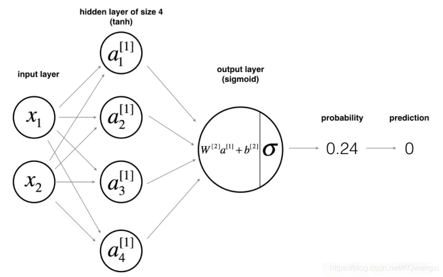
数学表达式：

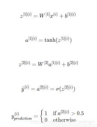
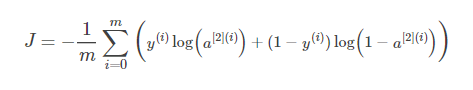
根据所有示例的预测，还可以按如下方式计算成本J：

提醒：建立神经网络的一般方法是：

定义神经网络结构（输入单元的#和隐藏单元的#等）。
初始化模型参数
构造回路：
- 实现前向传播
- 计算损失
- 实现反向传播以获得梯度
- 更新参数（梯度下降）

总之要将它们合并到一个我们称为nn_model（）的函数中。一旦构建了nn_model（）并学习了正确的参数，就可以对新数据进行预测。

4.1-定义神经网络结构

在构建神经网络之前，我们要先把神经网络的结构定义好：
定义三个变量：

n_x：输入层的数量
n_h：隐藏层的数量（设置为4）
n_y：输出层的数量

**提示：**使用X和Y的形状来查找n_x和n_y。另外，假设规定隐藏层的大小为4，即一层隐藏层有四个隐藏单元。

def layer_sizes(X , Y):
    """
    参数：
     X - 输入数据集,维度为（输入的数量，训练/测试的数量）
     Y - 标签，维度为（输出的数量，训练/测试数量）
    
    返回：
     n_x - 输入层的数量
     n_h - 隐藏层的数量
     n_y - 输出层的数量
    """
    n_x = X.shape[0] #输入层
    n_h = 4 #，隐藏层，硬编码为4
    n_y = Y.shape[0] #输出层
    
    return (n_x,n_h,n_y)

测试代码：

import numpy as np
import matplotlib.pyplot as plt
from testCases import *
import sklearn
import sklearn.datasets
import sklearn.linear_model
from planar_utils import plot_decision_boundary, sigmoid, load_planar_dataset, load_extra_datasets
np.random.seed(1) #设置一个固定的随机种子，以保证接下来的步骤中我们的结果是一致的。
X, Y = load_planar_dataset()


def layer_sizes(X, Y):
    """
    参数：
     X - 输入数据集,维度为（输入的数量，训练/测试的数量）
     Y - 标签，维度为（输出的数量，训练/测试数量）

    返回：
     n_x - 输入层的数量
     n_h - 隐藏层的数量
     n_y - 输出层的数量
    """
    n_x = X.shape[0]  # 输入层
    n_h = 4  # ，隐藏层，硬编码为4
    n_y = Y.shape[0]  # 输出层

    return (n_x, n_h, n_y)

#测试layer_sizes
print("=========================测试layer_sizes=========================")
X_asses , Y_asses = layer_sizes_test_case()
(n_x,n_h,n_y) =  layer_sizes(X_asses,Y_asses)
print("输入层的节点数量为: n_x = " + str(n_x))
print("隐藏层的节点数量为: n_h = " + str(n_h))
print("输出层的节点数量为: n_y = " + str(n_y))

运行结果：

=========================测试layer_sizes=========================
输入层的节点数量为: n_x = 5
隐藏层的节点数量为: n_h = 4
输出层的节点数量为: n_y = 2

4.2-初始化模型参数

练习：实现函数initialize\u parameters（）。
tips：

确保参数大小正确。如果需要，请参考上面的神经网络图。
需要使用随机值初始化权重矩阵。
- np.random.randn（a，b）*0.01随机初始化维度为（a，b）的矩阵，将偏移向量初始化为零。
- np.zeros（（a，b））用零初始化形状（a，b）的矩阵。

def initialize_parameters( n_x , n_h ,n_y):
    """
    参数：
        n_x - 输入层节点的数量
        n_h - 隐藏层节点的数量
        n_y - 输出层节点的数量
    
    返回：
        parameters - 包含参数的字典：
        W1 - 权重矩阵,维度为（n_h，n_x）
        b1 - 偏向量，维度为（n_h，1）
        W2 - 权重矩阵，维度为（n_y，n_h）
        b2 - 偏向量，维度为（n_y，1）

    """
    np.random.seed(2) #指定一个随机种子，以便你的输出与我们的一样。
    W1 = np.random.randn(n_h,n_x) * 0.01
    b1 = np.zeros(shape=(n_h, 1))
    W2 = np.random.randn(n_y,n_h) * 0.01
    b2 = np.zeros(shape=(n_y, 1))
    
    #使用断言确保我的数据格式是正确的
    assert(W1.shape == ( n_h , n_x ))
    assert(b1.shape == ( n_h , 1 ))
    assert(W2.shape == ( n_y , n_h ))
    assert(b2.shape == ( n_y , 1 ))
    
    parameters = {
    
    "W1" : W1,
	              "b1" : b1,
	              "W2" : W2,
	              "b2" : b2 }
    
    return parameters

测试代码：

#测试initialize_parameters
print("=========================测试initialize_parameters=========================")    
n_x , n_h , n_y = initialize_parameters_test_case()
parameters = initialize_parameters(n_x , n_h , n_y)
print("W1 = " + str(parameters["W1"]))
print("b1 = " + str(parameters["b1"]))
print("W2 = " + str(parameters["W2"]))
print("b2 = " + str(parameters["b2"]))

输出结果：

=========================测试initialize_parameters=========================
W1 = [[-0.00416758 -0.00056267]
 [-0.02136196  0.01640271]
 [-0.01793436 -0.00841747]
 [ 0.00502881 -0.01245288]]
b1 = [[ 0.]
 [ 0.]
 [ 0.]
 [ 0.]]
W2 = [[-0.01057952 -0.00909008  0.00551454  0.02292208]]
b2 = [[ 0.]]

4.3-构造回路

问题：实现前向传播

构造函数forward_propagation（）。
tips：

可以使用函数sigmoid（）。
你可以使用这个函数np.tanh(). 它是numpy库的一部分。

执行的步骤包括：

①使用字典类型的parameters（也就是**initializa_parameters( )**的输出）检索每个参数。
②实现正向传播。计算Z[1]、A[1]、Z[2]和A[2]（训练集中所有示例的预测向量）。
③反向传播所需的值存储在“cache”中，cache将作为反向传播函数的输入。

函数forward_propagation（）的实现：

def forward_propagation( X , parameters ):
    """
    参数：
         X - 维度为（n_x，m）的输入数据。
         parameters - 初始化函数（initialize_parameters）的输出
    
    返回：
         A2 - 使用sigmoid()函数计算的第二次激活后的数值
         cache - 包含“Z1”，“A1”，“Z2”和“A2”的字典类型变量
     """
    W1 = parameters["W1"]
    b1 = parameters["b1"]
    W2 = parameters["W2"]
    b2 = parameters["b2"]
    #前向传播计算A2
    Z1 = np.dot(W1 , X) + b1
    A1 = np.tanh(Z1)
    Z2 = np.dot(W2 , A1) + b2
    A2 = sigmoid(Z2)
    #使用断言确保我的数据格式是正确的
    assert(A2.shape == (1,X.shape[1]))
    cache = {
    
    "Z1": Z1,
             "A1": A1,
             "Z2": Z2,
             "A2": A2}
    
    return (A2, cache)

测试代码：

#测试forward_propagation
print("=========================测试forward_propagation=========================")
X_assess, parameters = forward_propagation_test_case()
A2, cache = forward_propagation(X_assess, parameters)
print(np.mean(cache["Z1"]), np.mean(cache["A1"]), np.mean(cache["Z2"]), np.mean(cache["A2"]))

输出结果：

=========================测试forward_propagation=========================
-0.000499755777742 -0.000496963353232 0.000438187450959 0.500109546852

4.4-计算成本函数

练习：实现compute_cost()来计算代价J的值。
在这里插入图片描述
交叉熵损失的实现方法有很多种，比如下述所示：

logprobs = np.multiply(np.log(A2),Y)
cost = - np.sum(logprobs)                # 不需要使用循环就可以直接算出来。

#构建计算成本的函数compute_cost()
def compute_cost(A2,Y,parameters):
    """
    按照上方提供的计算方程算出交叉熵成本，
    
    参数：
         A2 - 使用sigmoid()函数计算的第二次激活后的数值
         Y - "True"标签向量,维度为（1，数量）
         parameters - 一个包含W1，B1，W2和B2的字典类型的变量
    
    返回：
         成本 - 交叉熵成本给出方程（13）
    """
    
    m = Y.shape[1]
    W1 = parameters["W1"]
    W2 = parameters["W2"]
    
    #计算成本
    logprobs = np.multiply(np.log(A2), Y) + np.multiply((1 - Y), np.log(1 - A2))
    cost = -(1.0/m)*np.sum(logprobs)
    
    cost = np.squeeze(cost)
    #确保成本是我们期望的维度。
    assert(isinstance(cost,float))
    
    return cost

测试代码：

#测试compute_cost
print("=========================测试compute_cost=========================") 
A2 , Y_assess , parameters = compute_cost_test_case()
print("cost = " + str(compute_cost(A2,Y_assess,parameters)))

输出结果：

=========================测试compute_cost=========================
cost = 0.6929198937761266

使用前向传播期间计算的cache，现在可以利用它实现后向传播。

4.5-向后传播

反向传播通常是深度学习中最难(最数学化)的部分。为了帮助你们，这是关于反向传播的幻灯片。您将需要使用这张幻灯片右边的6个方程，因为您正在构建一个向量化的实现。
在这里插入图片描述
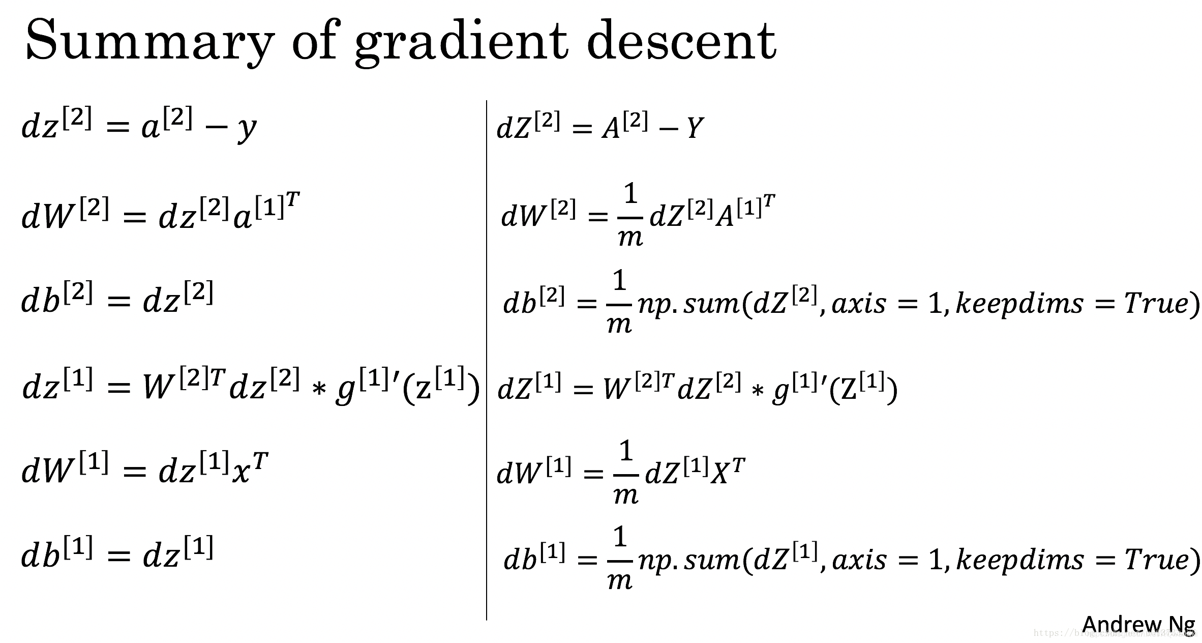
为了计算dZ^[1]，需要计算 g^[1]′(Z^[1])；
g^[1]’(……）是tanh激活函数，如果a = g^[1]’(z^[1] ) ,则g^[1]′(z)= 1-a²。
所以我们需要使用 (1 - np.power(A1, 2))来计算g^[1]′ (Z^[1]) 。

def backward_propagation(parameters,cache,X,Y):
    """
    使用上述说明搭建反向传播函数。
    
    参数：
     parameters - 包含我们的参数的一个字典类型的变量。
     cache - 包含“Z1”，“A1”，“Z2”和“A2”的字典类型的变量。
     X - 输入数据，维度为（2，数量）
     Y - “True”标签，维度为（1，数量）
    
    返回：
     grads - 包含W和b的导数的一个字典类型的变量。
    """
    m = X.shape[1]
    
    W1 = parameters["W1"]
    W2 = parameters["W2"]
    
    A1 = cache["A1"]
    A2 = cache["A2"]
    
    dZ2= A2 - Y
    dW2 = (1 / m) * np.dot(dZ2, A1.T)
    db2 = (1 / m) * np.sum(dZ2, axis=1, keepdims=True)
    dZ1 = np.multiply(np.dot(W2.T, dZ2), 1 - np.power(A1, 2))
    dW1 = (1 / m) * np.dot(dZ1, X.T)
    db1 = (1 / m) * np.sum(dZ1, axis=1, keepdims=True)
    grads = {
    
    "dW1": dW1,
             "db1": db1,
             "dW2": dW2,
             "db2": db2 }
    
    return grads

测试代码：

#测试backward_propagation
print("=========================测试backward_propagation=========================")
parameters, cache, X_assess, Y_assess = backward_propagation_test_case()

grads = backward_propagation(parameters, cache, X_assess, Y_assess)
print ("dW1 = "+ str(grads["dW1"]))
print ("db1 = "+ str(grads["db1"]))
print ("dW2 = "+ str(grads["dW2"]))
print ("db2 = "+ str(grads["db2"]))

输出结果：

=========================测试backward_propagation=========================
dW1 = [[ 0.01018708 -0.00708701]
 [ 0.00873447 -0.0060768 ]
 [-0.00530847  0.00369379]
 [-0.02206365  0.01535126]]
db1 = [[-0.00069728]
 [-0.00060606]
 [ 0.000364  ]
 [ 0.00151207]]
dW2 = [[ 0.00363613  0.03153604  0.01162914 -0.01318316]]
db2 = [[ 0.06589489]]

4.6-更新参数

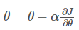
实现更新规则需要使用梯度下降法。而为了更新(W1, b1, W2, b2)，必须使用(dW1, db1, dW2, db2)。
一般梯度下降规则（α是学习速率，θ代表一个参数）:
在这里插入图片描述
我们需要选择一个良好的学习速率，我们可以看一下下面这两个图(由Adam Harley提供)
学习速率好的(收敛)

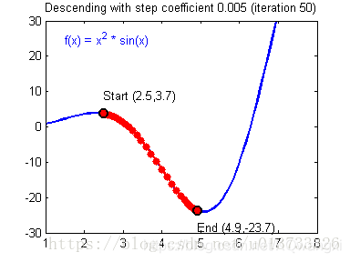
学习速率差的(发散)梯度下降算法：

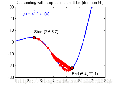
图片由Adam Harley提供。

def update_parameters(parameters,grads,learning_rate=1.2):
    """
    使用上面给出的梯度下降更新规则更新参数
    
    参数：
     parameters - 包含参数的字典类型的变量。
     grads - 包含导数值的字典类型的变量。
     learning_rate - 学习速率
    
    返回：
     parameters - 包含更新参数的字典类型的变量。
    """
    W1,W2 = parameters["W1"],parameters["W2"]
    b1,b2 = parameters["b1"],parameters["b2"]
    
    dW1,dW2 = grads["dW1"],grads["dW2"]
    db1,db2 = grads["db1"],grads["db2"]
    
    W1 = W1 - learning_rate * dW1
    b1 = b1 - learning_rate * db1
    W2 = W2 - learning_rate * dW2
    b2 = b2 - learning_rate * db2
    
    parameters = {
    
    "W1": W1,
                  "b1": b1,
                  "W2": W2,
                  "b2": b2}
    
    return parameters

测试代码：

测试一下update_parameters():

#测试update_parameters
print("=========================测试update_parameters=========================")
parameters, grads = update_parameters_test_case()
parameters = update_parameters(parameters, grads)

print("W1 = " + str(parameters["W1"]))
print("b1 = " + str(parameters["b1"]))
print("W2 = " + str(parameters["W2"]))
print("b2 = " + str(parameters["b2"]))

测试结果如下：



=========================测试update_parameters=========================
W1 = [[-0.00643025  0.01936718]
 [-0.02410458  0.03978052]
 [-0.01653973 -0.02096177]
 [ 0.01046864 -0.05990141]]
b1 = [[ -1.02420756e-06]
 [  1.27373948e-05]
 [  8.32996807e-07]
 [ -3.20136836e-06]]
W2 = [[-0.01041081 -0.04463285  0.01758031  0.04747113]]
b2 = [[ 0.00010457]]

4.7-整合

我们现在把上面的东西整合到nn_model()中，神经网络模型必须以正确的顺序使用先前的功能。

def nn_model(X,Y,n_h,num_iterations,print_cost=False):
    """
    参数：
        X - 数据集,维度为（2，示例数）
        Y - 标签，维度为（1，示例数）
        n_h - 隐藏层的数量
        num_iterations - 梯度下降循环中的迭代次数
        print_cost - 如果为True，则每1000次迭代打印一次成本数值
    
    返回：
        parameters - 模型学习的参数，它们可以用来进行预测。
     """
     
    np.random.seed(3) #指定随机种子
    n_x = layer_sizes(X, Y)[0]
    n_y = layer_sizes(X, Y)[2]
    
    parameters = initialize_parameters(n_x,n_h,n_y)
    W1 = parameters["W1"]
    b1 = parameters["b1"]
    W2 = parameters["W2"]
    b2 = parameters["b2"]
    
    for i in range(num_iterations):
        A2 , cache = forward_propagation(X,parameters)
        cost = compute_cost(A2,Y,parameters)
        grads = backward_propagation(parameters,cache,X,Y)
        parameters = update_parameters(parameters,grads,learning_rate = 0.5)
        
        if print_cost:
            if i%1000 == 0:
                print("第 ",i," 次循环，成本为："+str(cost))
    return parameters

测试nn_model():

#测试nn_model
print("=========================测试nn_model=========================")
X_assess, Y_assess = nn_model_test_case()

parameters = nn_model(X_assess, Y_assess, 4, num_iterations=10000, print_cost=True)
print("W1 = " + str(parameters["W1"]))
print("b1 = " + str(parameters["b1"]))
print("W2 = " + str(parameters["W2"]))
print("b2 = " + str(parameters["b2"]))

输出：

W1 = [[-3.89167767  4.77541602]
 [-6.77960338  1.20272585]
 [-3.88338966  4.78028666]
 [ 6.77958203 -1.20272574]]
b1 = [[ 2.11530892]
 [ 3.41221357]
 [ 2.11585732]
 [-3.41221322]]
W2 = [[-2512.9093032  -2502.70799785 -2512.01655969  2502.65264416]]
b2 = [[-22.29071761]]

参数更新完了我们就可以来进行预测了。

4.8-预测

通过构建predict()来使用您的模型进行预测。并使用正向传播来预测结果。
提示:
predictions = Ypredict

=1{activation >0.5}
=0{if 0.5>activation>0}
例如，如果您希望根据阈值将矩阵X的条目设置为0和1，您可以这样做:X_new = (X > threshold)

def predict(parameters,X):
    """
    使用学习的参数，为X中的每个示例预测一个类
    
    参数：
		parameters - 包含参数的字典类型的变量。
	    X - 输入数据（n_x，m）
    
    返回
		predictions - 我们模型预测的向量（红色：0 /蓝色：1）
     
     """
    A2 , cache = forward_propagation(X,parameters)
    predictions = np.round(A2)
    
    return predictions

#测试predict
print("=========================测试predict=========================")

parameters, X_assess = predict_test_case()

predictions = predict(parameters, X_assess)
print("预测的平均值 = " + str(np.mean(predictions)))

=========================测试predict=========================
预测的平均值 = 0.666666666667

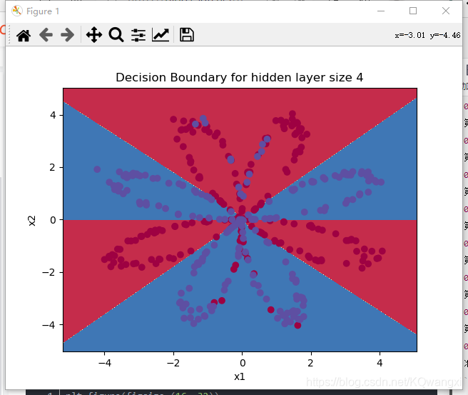
4.9-运行代码

parameters = nn_model(X, Y, n_h = 4, num_iterations=10000, print_cost=True)

#绘制边界
plot_decision_boundary(lambda x: predict(parameters, x.T), X, Y)
plt.title("Decision Boundary for hidden layer size " + str(4))
plt.show()
predictions = predict(parameters, X)
print ('准确率: %d' % float((np.dot(Y, predictions.T) + np.dot(1 - Y, 1 - predictions.T)) / float(Y.size) * 100) + '%')

第  0  次循环，成本为：0.6930480201239823
第  1000  次循环，成本为：0.3098018601352803
第  2000  次循环，成本为：0.2924326333792647
第  3000  次循环，成本为：0.2833492852647411
第  4000  次循环，成本为：0.27678077562979253
第  5000  次循环，成本为：0.2634715508859307
第  6000  次循环，成本为：0.24204413129940758
第  7000  次循环，成本为：0.23552486626608762
第  8000  次循环，成本为：0.23140964509854278
第  9000  次循环，成本为：0.22846408048352362
准确率: 90%

在这里插入图片描述

4.10 更改隐藏层节点数量

我们上面的实验把隐藏层定为4个节点，现在我们更改隐藏层里面的节点数量，看一看节点数量是否会对结果造成影响。

plt.figure(figsize=(16, 32))
hidden_layer_sizes = [1, 2, 3, 4, 5, 20, 50] #隐藏层数量
for i, n_h in enumerate(hidden_layer_sizes):
    plt.subplot(5, 2, i + 1)
    plt.title('Hidden Layer of size %d' % n_h)
    parameters = nn_model(X, Y, n_h, num_iterations=5000)
    plot_decision_boundary(lambda x: predict(parameters, x.T), X, Y)
    predictions = predict(parameters, X)
    accuracy = float((np.dot(Y, predictions.T) + np.dot(1 - Y, 1 - predictions.T)) / float(Y.size) * 100)
    print ("隐藏层的节点数量： {}  ，准确率: {} %".format(n_h, accuracy))
    pass
plt.show()

打印结果

D:\Adobe\Anaconda3\python.exe D:/code/dataClassification/code/test.py
第  0  次循环，成本为：0.6930480201239823
第  1000  次循环，成本为：0.3098018601352803
第  2000  次循环，成本为：0.2924326333792647
第  3000  次循环，成本为：0.2833492852647411
第  4000  次循环，成本为：0.27678077562979253
第  5000  次循环，成本为：0.2634715508859307
第  6000  次循环，成本为：0.24204413129940758
第  7000  次循环，成本为：0.23552486626608762
第  8000  次循环，成本为：0.23140964509854278
第  9000  次循环，成本为：0.22846408048352362
隐藏层的节点数量： 1  ，准确率: 67.25 %
隐藏层的节点数量： 2  ，准确率: 66.5 %
隐藏层的节点数量： 3  ，准确率: 89.25 %
隐藏层的节点数量： 4  ，准确率: 90.0 %
隐藏层的节点数量： 5  ，准确率: 89.75 %
隐藏层的节点数量： 20  ，准确率: 90.0 %
隐藏层的节点数量： 50  ，准确率: 89.75 %

在这里插入图片描述
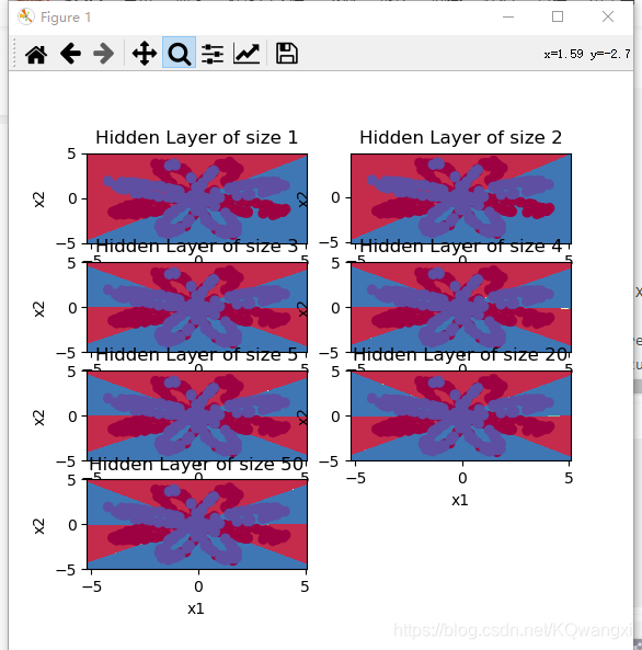
较大的模型（具有更多隐藏单元）能够更好地适应训练集，直到最终的最大模型过度拟合数据。
最好的隐藏层大小似乎在n_h = 5附近。实际上，这里的值似乎很适合数据，而且不会引起过度拟合。
我们还将在后面学习有关正则化的知识，它允许我们使用非常大的模型（如n_h = 50），而不会出现太多过度拟合。

4.11【选做】</span

当改变sigmoid激活或ReLU激活的tanh激活时会发生什么？
改变learning_rate的数值会发生什么
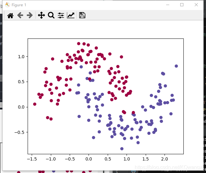
如果我们改变数据集呢？

# 数据集
noisy_circles, noisy_moons, blobs, gaussian_quantiles, no_structure = load_extra_datasets()

datasets = {
    
    "noisy_circles": noisy_circles,
            "noisy_moons": noisy_moons,
            "blobs": blobs,
            "gaussian_quantiles": gaussian_quantiles}

dataset = "noisy_moons"

X, Y = datasets[dataset]
X, Y = X.T, Y.reshape(1, Y.shape[0])

if dataset == "blobs":
    Y = Y % 2

plt.scatter(X[0, :], X[1, :], c=Y, s=40, cmap=plt.cm.Spectral)

#上一语句如出现问题请使用下面的语句：
plt.scatter(X[0, :], X[1, :], c=np.squeeze(Y), s=40, cmap=plt.cm.Spectral)

在这里插入图片描述

第五部分:完整代码

import numpy as np
import matplotlib.pyplot as plt
from testCases import *
import sklearn
import sklearn.datasets
import sklearn.linear_model
from planar_utils import plot_decision_boundary, sigmoid, load_planar_dataset, load_extra_datasets
np.random.seed(1) #设置一个固定的随机种子，以保证接下来的步骤中我们的结果是一致的。
X, Y = load_planar_dataset()

def layer_sizes(X, Y):
    """
    参数：
     X - 输入数据集,维度为（输入的数量，训练/测试的数量）
     Y - 标签，维度为（输出的数量，训练/测试数量）

    返回：
     n_x - 输入层的数量
     n_h - 隐藏层的数量
     n_y - 输出层的数量
    """
    n_x = X.shape[0]  # 输入层
    n_h = 4  # ，隐藏层，硬编码为4
    n_y = Y.shape[0]  # 输出层

    return (n_x, n_h, n_y)
def initialize_parameters(n_x, n_h, n_y):
    """
    参数：
        n_x - 输入层节点的数量
        n_h - 隐藏层节点的数量
        n_y - 输出层节点的数量

    返回：
        parameters - 包含参数的字典：
            W1 - 权重矩阵,维度为（n_h，n_x）
            b1 - 偏向量，维度为（n_h，1）
            W2 - 权重矩阵，维度为（n_y，n_h）
            b2 - 偏向量，维度为（n_y，1）

    """
    np.random.seed(2)  # 指定一个随机种子，以便你的输出与我们的一样。
    W1 = np.random.randn(n_h, n_x) * 0.01
    b1 = np.zeros(shape=(n_h, 1))
    W2 = np.random.randn(n_y, n_h) * 0.01
    b2 = np.zeros(shape=(n_y, 1))

    # 使用断言确保我的数据格式是正确的
    assert (W1.shape == (n_h, n_x))
    assert (b1.shape == (n_h, 1))
    assert (W2.shape == (n_y, n_h))
    assert (b2.shape == (n_y, 1))

    parameters = {
    
    "W1": W1,
                  "b1": b1,
                  "W2": W2,
                  "b2": b2}

    return parameters
def forward_propagation(X, parameters):
    """
    参数：
         X - 维度为（n_x，m）的输入数据。
         parameters - 初始化函数（initialize_parameters）的输出

    返回：
         A2 - 使用sigmoid()函数计算的第二次激活后的数值
         cache - 包含“Z1”，“A1”，“Z2”和“A2”的字典类型变量
     """
    W1 = parameters["W1"]
    b1 = parameters["b1"]
    W2 = parameters["W2"]
    b2 = parameters["b2"]
    # 前向传播计算A2
    Z1 = np.dot(W1, X) + b1
    A1 = np.tanh(Z1)
    Z2 = np.dot(W2, A1) + b2
    A2 = sigmoid(Z2)
    # 使用断言确保我的数据格式是正确的
    assert (A2.shape == (1, X.shape[1]))
    cache = {
    
    "Z1": Z1,
             "A1": A1,
             "Z2": Z2,
             "A2": A2}

    return (A2, cache)
def compute_cost(A2, Y, parameters):
    """
    计算方程（6）中给出的交叉熵成本，

    参数：
         A2 - 使用sigmoid()函数计算的第二次激活后的数值
         Y - "True"标签向量,维度为（1，数量）
         parameters - 一个包含W1，B1，W2和B2的字典类型的变量

    返回：
         成本 - 交叉熵成本给出方程（13）
    """

    m = Y.shape[1]
    W1 = parameters["W1"]
    W2 = parameters["W2"]

    # 计算成本
    logprobs = np.multiply(np.log(A2),Y) + np.multiply(np.log(1-A2), (1-Y))
    cost = -(1.0 / m) * np.sum(logprobs)
    cost = np.squeeze(cost)

    assert (isinstance(cost, float))

    return cost
def backward_propagation(parameters, cache, X, Y):
    """
    使用上述说明搭建反向传播函数。

    参数：
     parameters - 包含我们的参数的一个字典类型的变量。
     cache - 包含“Z1”，“A1”，“Z2”和“A2”的字典类型的变量。
     X - 输入数据，维度为（2，数量）
     Y - “True”标签，维度为（1，数量）

    返回：
     grads - 包含W和b的导数一个字典类型的变量。
    """
    m = X.shape[1]

    W1 = parameters["W1"]
    W2 = parameters["W2"]

    A1 = cache["A1"]
    A2 = cache["A2"]

    dZ2 = A2 - Y
    dW2 = (1 / m) * np.dot(dZ2, A1.T)
    db2 = (1 / m) * np.sum(dZ2, axis=1, keepdims=True)
    dZ1 = np.multiply(np.dot(W2.T, dZ2), 1 - np.power(A1, 2))
    dW1 = (1 / m) * np.dot(dZ1, X.T)
    db1 = (1 / m) * np.sum(dZ1, axis=1, keepdims=True)
    grads = {
    
    "dW1": dW1,
             "db1": db1,
             "dW2": dW2,
             "db2": db2}

    return grads
def update_parameters(parameters, grads, learning_rate=1.2):
    """
    使用上面给出的梯度下降更新规则更新参数

    参数：
     parameters - 包含参数的字典类型的变量。
     grads - 包含导数值的字典类型的变量。
     learning_rate - 学习速率

    返回：
     parameters - 包含更新参数的字典类型的变量。
    """
    W1, W2 = parameters["W1"], parameters["W2"]
    b1, b2 = parameters["b1"], parameters["b2"]

    dW1, dW2 = grads["dW1"], grads["dW2"]
    db1, db2 = grads["db1"], grads["db2"]

    W1 = W1 - learning_rate * dW1
    b1 = b1 - learning_rate * db1
    W2 = W2 - learning_rate * dW2
    b2 = b2 - learning_rate * db2

    parameters = {
    
    "W1": W1,
                  "b1": b1,
                  "W2": W2,
                  "b2": b2}

    return parameters

def nn_model(X, Y, n_h, num_iterations, print_cost=False):
    """
    参数：
        X - 数据集,维度为（2，示例数）
        Y - 标签，维度为（1，示例数）
        n_h - 隐藏层的数量
        num_iterations - 梯度下降循环中的迭代次数
        print_cost - 如果为True，则每1000次迭代打印一次成本数值

    返回：
        parameters - 模型学习的参数，它们可以用来进行预测。
     """

    np.random.seed(3)  # 指定随机种子
    n_x = layer_sizes(X, Y)[0]
    n_y = layer_sizes(X, Y)[2]

    parameters = initialize_parameters(n_x, n_h, n_y)
    W1 = parameters["W1"]
    b1 = parameters["b1"]
    W2 = parameters["W2"]
    b2 = parameters["b2"]

    for i in range(num_iterations):
        A2, cache = forward_propagation(X, parameters)
        cost = compute_cost(A2, Y, parameters)
        grads = backward_propagation(parameters, cache, X, Y)
        parameters = update_parameters(parameters, grads, learning_rate=0.5)

        if print_cost:
            if i % 1000 == 0:
                print("第 ", i, " 次循环，成本为：" + str(cost))
    return parameters


def predict(parameters, X):
    """
    使用学习的参数，为X中的每个示例预测一个类

    参数：
		parameters - 包含参数的字典类型的变量。
	    X - 输入数据（n_x，m）

    返回
		predictions - 我们模型预测的向量（红色：0 /蓝色：1）

     """
    A2, cache = forward_propagation(X, parameters)
    predictions = np.round(A2)

    return predictions



parameters = nn_model(X, Y, n_h = 4, num_iterations=10000, print_cost=True)
#绘制边界
plot_decision_boundary(lambda x: predict(parameters, x.T), X, Y)
plt.title("Decision Boundary for hidden layer size " + str(4))
plt.show()
predictions = predict(parameters, X)
print ('准确率: %d' % float((np.dot(Y, predictions.T) + np.dot(1 - Y, 1 - predictions.T)) / float(Y.size) * 100) + '%')

"""
plt.figure(figsize=(16, 32))
hidden_layer_sizes = [1, 2, 3, 4, 5, 20, 50] #隐藏层数量
for i, n_h in enumerate(hidden_layer_sizes):
    plt.subplot(5, 2, i + 1)
    plt.title('Hidden Layer of size %d' % n_h)
    parameters = nn_model(X, Y, n_h, num_iterations=5000)
    plot_decision_boundary(lambda x: predict(parameters, x.T), X, Y)
    predictions = predict(parameters, X)
    accuracy = float((np.dot(Y, predictions.T) + np.dot(1 - Y, 1 - predictions.T)) / float(Y.size) * 100)
    print ("隐藏层的节点数量： {}  ，准确率: {} %".format(n_h, accuracy))
    pass
plt.show()
"""

第六部分:testCases.py文件内容

#-*- coding: UTF-8 -*-
"""
# WANGZHE12
"""
import numpy as np

def layer_sizes_test_case():
    np.random.seed(1)
    X_assess = np.random.randn(5, 3)
    Y_assess = np.random.randn(2, 3)
    return X_assess, Y_assess

def initialize_parameters_test_case():
    n_x, n_h, n_y = 2, 4, 1
    return n_x, n_h, n_y

def forward_propagation_test_case():
    np.random.seed(1)
    X_assess = np.random.randn(2, 3)

    parameters = {
    
    'W1': np.array([[-0.00416758, -0.00056267],
        [-0.02136196,  0.01640271],
        [-0.01793436, -0.00841747],
        [ 0.00502881, -0.01245288]]),
     'W2': np.array([[-0.01057952, -0.00909008,  0.00551454,  0.02292208]]),
     'b1': np.array([[ 0.],
        [ 0.],
        [ 0.],
        [ 0.]]),
     'b2': np.array([[ 0.]])}

    return X_assess, parameters

def compute_cost_test_case():
    np.random.seed(1)
    Y_assess = np.random.randn(1, 3)
    parameters = {
    
    'W1': np.array([[-0.00416758, -0.00056267],
        [-0.02136196,  0.01640271],
        [-0.01793436, -0.00841747],
        [ 0.00502881, -0.01245288]]),
     'W2': np.array([[-0.01057952, -0.00909008,  0.00551454,  0.02292208]]),
     'b1': np.array([[ 0.],
        [ 0.],
        [ 0.],
        [ 0.]]),
     'b2': np.array([[ 0.]])}

    a2 = (np.array([[ 0.5002307 ,  0.49985831,  0.50023963]]))

    return a2, Y_assess, parameters

def backward_propagation_test_case():
    np.random.seed(1)
    X_assess = np.random.randn(2, 3)
    Y_assess = np.random.randn(1, 3)
    parameters = {
    
    'W1': np.array([[-0.00416758, -0.00056267],
        [-0.02136196,  0.01640271],
        [-0.01793436, -0.00841747],
        [ 0.00502881, -0.01245288]]),
     'W2': np.array([[-0.01057952, -0.00909008,  0.00551454,  0.02292208]]),
     'b1': np.array([[ 0.],
        [ 0.],
        [ 0.],
        [ 0.]]),
     'b2': np.array([[ 0.]])}

    cache = {
    
    'A1': np.array([[-0.00616578,  0.0020626 ,  0.00349619],
         [-0.05225116,  0.02725659, -0.02646251],
         [-0.02009721,  0.0036869 ,  0.02883756],
         [ 0.02152675, -0.01385234,  0.02599885]]),
  'A2': np.array([[ 0.5002307 ,  0.49985831,  0.50023963]]),
  'Z1': np.array([[-0.00616586,  0.0020626 ,  0.0034962 ],
         [-0.05229879,  0.02726335, -0.02646869],
         [-0.02009991,  0.00368692,  0.02884556],
         [ 0.02153007, -0.01385322,  0.02600471]]),
  'Z2': np.array([[ 0.00092281, -0.00056678,  0.00095853]])}
    return parameters, cache, X_assess, Y_assess

def update_parameters_test_case():
    parameters = {
    
    'W1': np.array([[-0.00615039,  0.0169021 ],
        [-0.02311792,  0.03137121],
        [-0.0169217 , -0.01752545],
        [ 0.00935436, -0.05018221]]),
 'W2': np.array([[-0.0104319 , -0.04019007,  0.01607211,  0.04440255]]),
 'b1': np.array([[ -8.97523455e-07],
        [  8.15562092e-06],
        [  6.04810633e-07],
        [ -2.54560700e-06]]),
 'b2': np.array([[  9.14954378e-05]])}

    grads = {
    
    'dW1': np.array([[ 0.00023322, -0.00205423],
        [ 0.00082222, -0.00700776],
        [-0.00031831,  0.0028636 ],
        [-0.00092857,  0.00809933]]),
 'dW2': np.array([[ -1.75740039e-05,   3.70231337e-03,  -1.25683095e-03,
          -2.55715317e-03]]),
 'db1': np.array([[  1.05570087e-07],
        [ -3.81814487e-06],
        [ -1.90155145e-07],
        [  5.46467802e-07]]),
 'db2': np.array([[ -1.08923140e-05]])}
    return parameters, grads

def nn_model_test_case():
    np.random.seed(1)
    X_assess = np.random.randn(2, 3)
    Y_assess = np.random.randn(1, 3)
    return X_assess, Y_assess

def predict_test_case():
    np.random.seed(1)
    X_assess = np.random.randn(2, 3)
    parameters = {
    
    'W1': np.array([[-0.00615039,  0.0169021 ],
        [-0.02311792,  0.03137121],
        [-0.0169217 , -0.01752545],
        [ 0.00935436, -0.05018221]]),
     'W2': np.array([[-0.0104319 , -0.04019007,  0.01607211,  0.04440255]]),
     'b1': np.array([[ -8.97523455e-07],
        [  8.15562092e-06],
        [  6.04810633e-07],
        [ -2.54560700e-06]]),
     'b2': np.array([[  9.14954378e-05]])}
    return parameters, X_assess

第七部分:planar_utils.py文件内容

import matplotlib.pyplot as plt
import numpy as np
import sklearn
import sklearn.datasets
import sklearn.linear_model

def plot_decision_boundary(model, X, y):
    # Set min and max values and give it some padding
    x_min, x_max = X[0, :].min() - 1, X[0, :].max() + 1
    y_min, y_max = X[1, :].min() - 1, X[1, :].max() + 1
    h = 0.01
    # Generate a grid of points with distance h between them
    xx, yy = np.meshgrid(np.arange(x_min, x_max, h), np.arange(y_min, y_max, h))
    # Predict the function value for the whole grid
    Z = model(np.c_[xx.ravel(), yy.ravel()])
    Z = Z.reshape(xx.shape)
    # Plot the contour and training examples
    plt.contourf(xx, yy, Z, cmap=plt.cm.Spectral)
    plt.ylabel('x2')
    plt.xlabel('x1')
    plt.scatter(X[0, :], X[1, :], c=y, cmap=plt.cm.Spectral)


def sigmoid(x):
    s = 1/(1+np.exp(-x))
    return s

def load_planar_dataset():
    np.random.seed(1)
    m = 400 # number of examples
    N = int(m/2) # number of points per class
    D = 2 # dimensionality
    X = np.zeros((m,D)) # data matrix where each row is a single example
    Y = np.zeros((m,1), dtype='uint8') # labels vector (0 for red, 1 for blue)
    a = 4 # maximum ray of the flower

    for j in range(2):
        ix = range(N*j,N*(j+1))
        t = np.linspace(j*3.12,(j+1)*3.12,N) + np.random.randn(N)*0.2 # theta
        r = a*np.sin(4*t) + np.random.randn(N)*0.2 # radius
        X[ix] = np.c_[r*np.sin(t), r*np.cos(t)]
        Y[ix] = j

    X = X.T
    Y = Y.T

    return X, Y

def load_extra_datasets():  
    N = 200
    noisy_circles = sklearn.datasets.make_circles(n_samples=N, factor=.5, noise=.3)
    noisy_moons = sklearn.datasets.make_moons(n_samples=N, noise=.2)
    blobs = sklearn.datasets.make_blobs(n_samples=N, random_state=5, n_features=2, centers=6)
    gaussian_quantiles = sklearn.datasets.make_gaussian_quantiles(mean=None, cov=0.5, n_samples=N, n_features=2, n_classes=2, shuffle=True, random_state=None)
    no_structure = np.random.rand(N, 2), np.random.rand(N, 2)

    return noisy_circles, noisy_moons, blobs, gaussian_quantiles, no_structure

“吴恩达深度学习”第三周编程代码汇总（实现一个神经网络）

前言

目录

第一部分:需要准备的Packages

第2部分:加载和查看数据集

第3部分:查看简单的Logistic回归的分类效果

第四部分:搭建神经网络

4.1-定义神经网络结构

4.2-初始化模型参数

4.3-构造回路

4.4-计算成本函数

4.5-向后传播

4.6-更新参数

4.7-整合

4.8-预测

4.9-运行代码

4.10 更改隐藏层节点数量

4.11【选做】</span

第五部分:完整代码

第六部分:testCases.py文件内容

第七部分:planar_utils.py文件内容

猜你喜欢