Matlab之图像变换技术（十二）

图像变换是将图像从空间域变换到变换域。图像变换的目的是根据图像在变换域的某些性质对其进行处理。通常，这些性质在空间城内很难获取。在变换城内处理结束后，将处理结果进行反变换到空间城。

这里将详细介紹图像变换技术，主要包括Radon变换和反变换，傅立叶变换和反变换，离散余弦变换和反变换等。

---

人类视觉所看到的图像是在空域上的，其信息具有很强的相关性，所以经常将图像信号通过某种数学方法变换到其它正交矢量空间上。一般称原始图像为空间域图像，称变换后的图像为变换域图像，变换域图像可反变换为空间域图像。

图像RADON变换

在进行二维或三维投影数据重建时，图像重建方法虽然很多，但是通常采用Radon变换和Radon反变换作为基础。

RADON正变换

在MATLAB软件中，采用函数radon( )进行图像的Radon变换，该函数的调用格式为：

R = radon(I, theta)
%该函数对图像I进行Radon变换，theta为角度，函数的返回值R为图像I在theta方向上的变换值。

[R, xp] = radon(...)
%该函数的返回值xp为对应的坐标值。

举个例子

clear all;
close all;
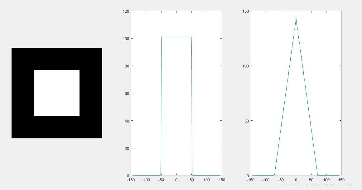
I = zeros(200, 200);
I(50:150, 50: 150) = 1;
[R, xp] = radon(I, [0, 45]);

figure;
subplot(131), imshow(I);
subplot(132), plot(xp, R(:, 1));
subplot(133), plot(xp, R(:, 2));

分别绘制0度和45度的Radon变换

clear all;
close all;
I = zeros(200, 200);
I(50:150, 50: 150) = 1;
theta = 0: 10: 180;
[R, xp] = radon(I, theta);

figure;
subplot(121), imshow(I);
subplot(122), imagesc(theta, xp, R);
colormap(hot);
colorbar;

角度每隔10度做radon变换再绘制到一起，

clear all;
close all;
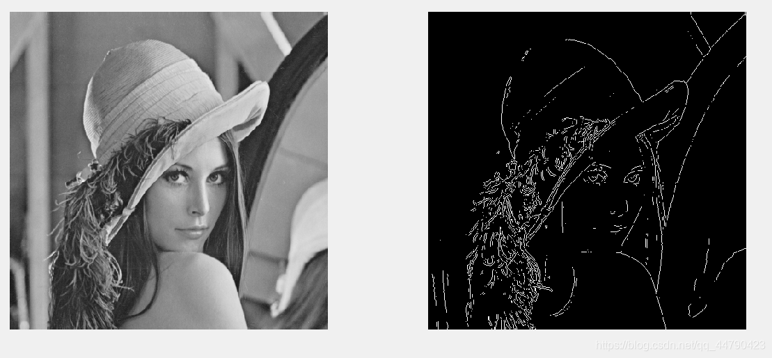
I = imread('lena_color_512.tif');
J = rgb2gray(I);
BW = edge(J);
figure;
subplot(121), imshow(J);
subplot(122), imshow(BW);

theta = 0: 179;
[R, xp] = radon(BW, theta);

figure;
imagesc(theta, xp, R);
colormap(hot);
colorbar;

Rmax = max(max(R))
[row, column] = find(R >= Rmax)
x = xp(row)
angel = theta(column)

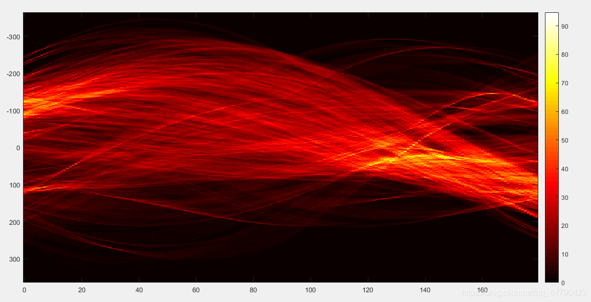
Rmax =
   94.7542
row =
   393
column =
   150
x =
    28
angel =
   149

Radon反变换

在MATLAB软件中， 采用函数iradon( )计算Radon反变换，该函数的调用格式为：

I = iradon(R, theta)
%该函数进行Radon反变换，R为Radon变换矩阵，theta为角度，函数的返回值I为反变换后得到的图像。

举个例子

clear all;
close all;
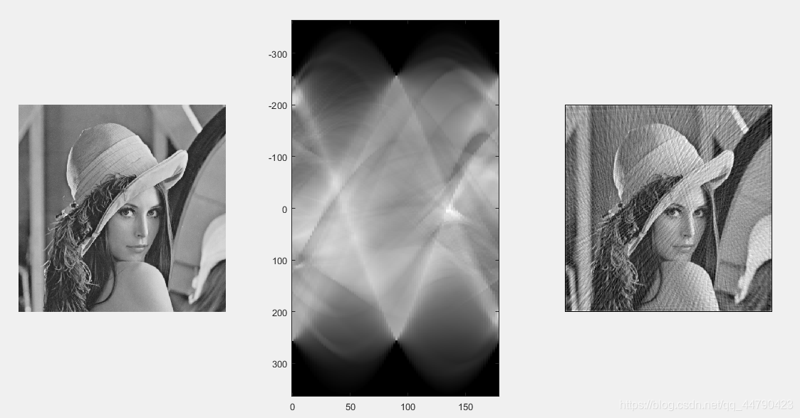
I = imread('lena_color_512.tif');
I = rgb2gray(I);

theta = 0: 2: 179;
[R, xp] = radon(I, theta);
J = iradon(R, theta);

figure;
subplot(131), imshow(uint8(I));
subplot(132), imagesc(theta, xp, R);
axis normal;
subplot(133), imshow(uint8(J));

左边为原图，中间是radon结果，右边是iradon的结果

图像傅里叶变换

在MATLAB软件中，通过函数fft( )进行一维离散傅立叶变换，通过函数ifft( )进行一维离散傅立叶反变换。函数fff( )和ifft( )的详细使用情况，可自己查询MATLAB的帮助系统。在MATLAB中，采用函数fft2( )进行二维离散傅立叶变换，函数fft( )和fft2( )的关系为fft2(X) = fft(fft(X).’ ).’ 。
函数fft2( )的详细调用情况如下所示：

Y = fft2(X)
%该函数采用快速FFT算法，计算矩阵X的二维离散傅立叶变换，结果返回给Y，Y的大小与X相同。
Y = fft2(X, m,n)
%该函数采用快速FFT算法，计算矩阵大小为m*n的二维离散傅立叶变换

举个栗子

clear all;
close all;
I = imread('lena_color_512.tif');
I = rgb2gray(I);

J = fft2(I);
K = abs(J/256);

figure;
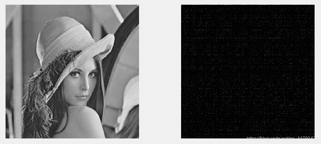
subplot(121), imshow(I);
subplot(122), imshow(uint8(K));

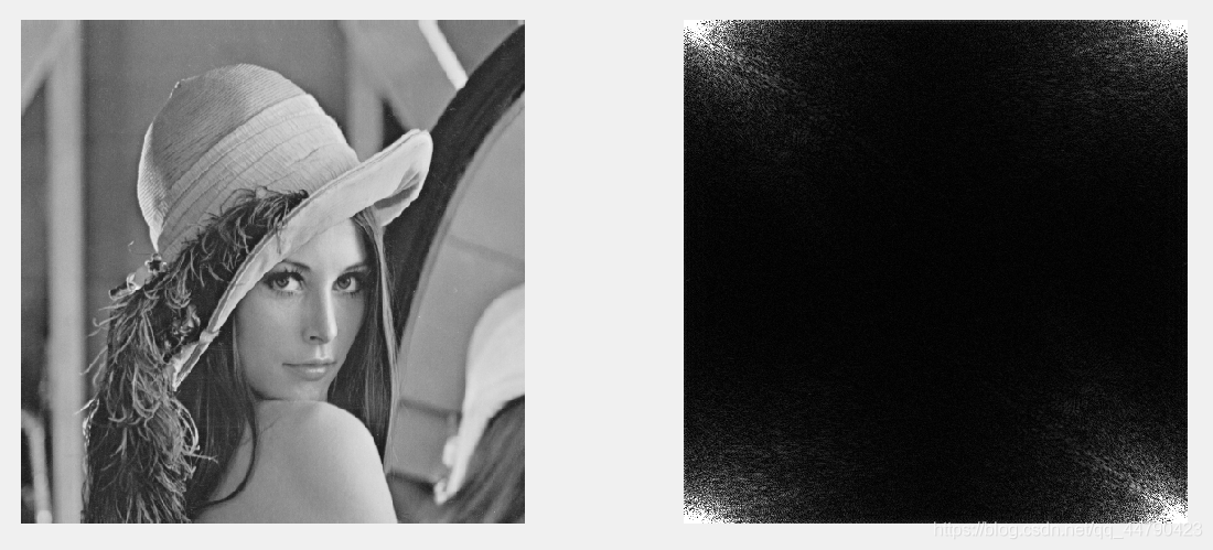
对于该频谱图，左上角为坐标原点，其余四个角为低频成分，故我们尝试把其频域到中心去

clear all;
close all;
I = imread('lena_color_512.tif');
J = rgb2gray(I);

K = fft2(J);
K = fftshift(K);  %频移
L = abs(K/256);


figure;
subplot(121), imshow(J);
subplot(122), imshow(uint8(L));

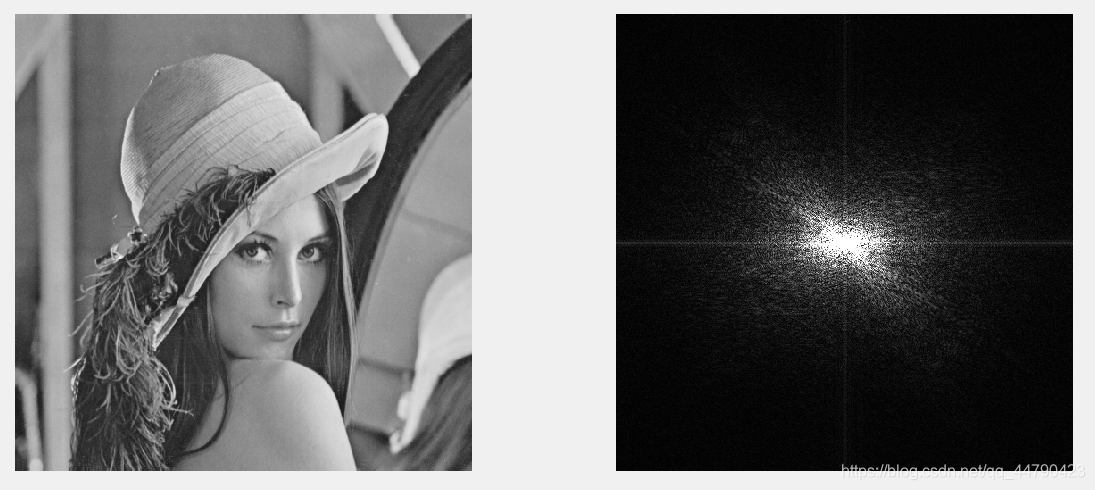
使频谱图像白色增多

clear all;
close all;
I = imread('lena_color_512.tif');
J = rgb2gray(I);

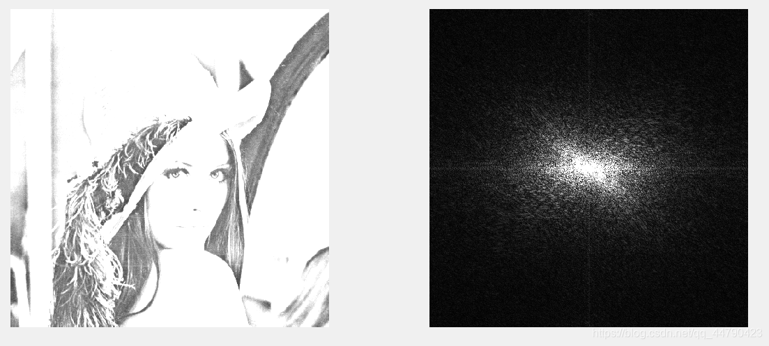
J = J*exp(1);
J(find(J>255)) = 255; %使变亮
K = fft2(J);
K = fftshift(K);  %频移
L = abs(K/256);

figure;
subplot(121), imshow(J);
subplot(122), imshow(uint8(L));

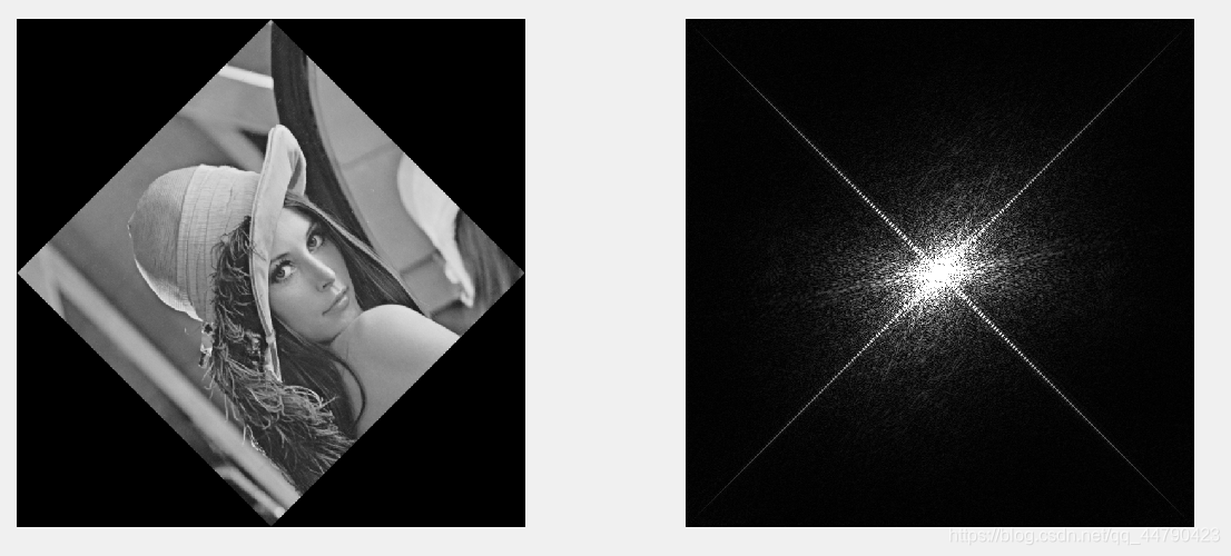
旋转图形，观察频谱图

clear all;
close all;
I = imread('lena_color_512.tif');
J = rgb2gray(I);

J = imrotate(J, 45, 'bilinear');%旋转
K = fft2(J);
K = fftshift(K);  %频移
L = abs(K/256);

figure;
subplot(121), imshow(J);
subplot(122), imshow(uint8(L));

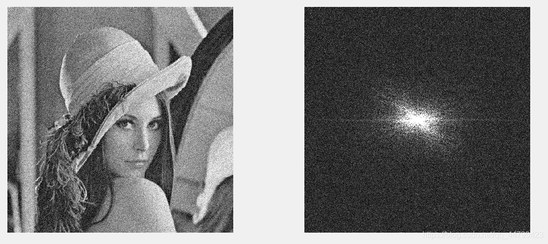
给图像加噪之后的频谱图

clear all;
close all;
I = imread('lena_color_512.tif');
J = rgb2gray(I);

J = imnoise(J, 'gaussian', 0, 0.01);%加高斯噪声
K = fft2(J);
K = fftshift(K);  %频移
L = abs(K/256);

figure;
subplot(121), imshow(J);
subplot(122), imshow(uint8(L));

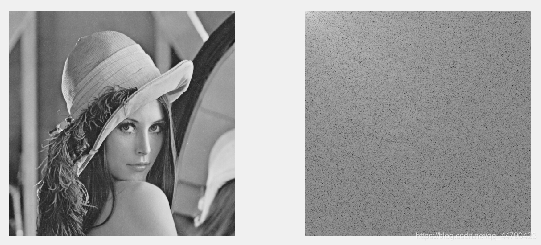
图像离散余弦变换

离散余弦变换是以一组不同频率和幅值的余弦西数和来近似一幅图像，实际上是傅立叶变换的实数部分。离散余弦变换(Discrete Cosine Transform,DCT)有一个重要的性质，即对于一幅图像，其大部分可视化信息都集中在少数的变换系数上。因此，离散余弦变换经常用于图像压缩。

在MATLAB软件中，采用函数dct( )进行一维离散余弦变换，采用函数idct()进行一维离散余弦反变换，通过函数dct2( )进行二维离散余弦变换，该函数的详细使用情况如下所示：

B = dct2(A)
%该函数计算图像矩阵A的二维离散余弦变换，返回值为B, A和B的大小相同。

B = dct2(A, m, n)或B= dct2(A, [m, n])
% 该函数计算图像矩阵A的二维离散余弦变换，返回值为B,通过对A补0或剪裁，使得B的大小为m行n列。

举个栗子

clear all;
close all;
I = imread('lena_color_512.tif');
I = rgb2gray(I);
I = im2double(I);
J = dct2(I);

figure;
subplot(121), imshow(I);
subplot(122), imshow(log(abs(J)), []);

可知能量主要集中在左上角，其余的系数近似为0

实验dct2

• 构造离散余弦函数矩阵

clear all;
close all;

A = [1 1 1 1; 2 2 2 2; 3 3 3 3]
s = size(A);
M = s(1);
N = s(2);
P = dctmtx(M)
Q = dctmtx(N)
B = P*A*Q'

%结果
A =
     1     1     1     1
     2     2     2     2
     3     3     3     3
P =
    0.5774    0.5774    0.5774
    0.7071    0.0000   -0.7071
    0.4082   -0.8165    0.4082
Q =
    0.5000    0.5000    0.5000    0.5000
    0.6533    0.2706   -0.2706   -0.6533
    0.5000   -0.5000   -0.5000    0.5000
    0.2706   -0.6533    0.6533   -0.2706
B =
    6.9282         0   -0.0000   -0.0000
   -2.8284         0    0.0000    0.0000
    0.0000         0   -0.0000   -0.0000

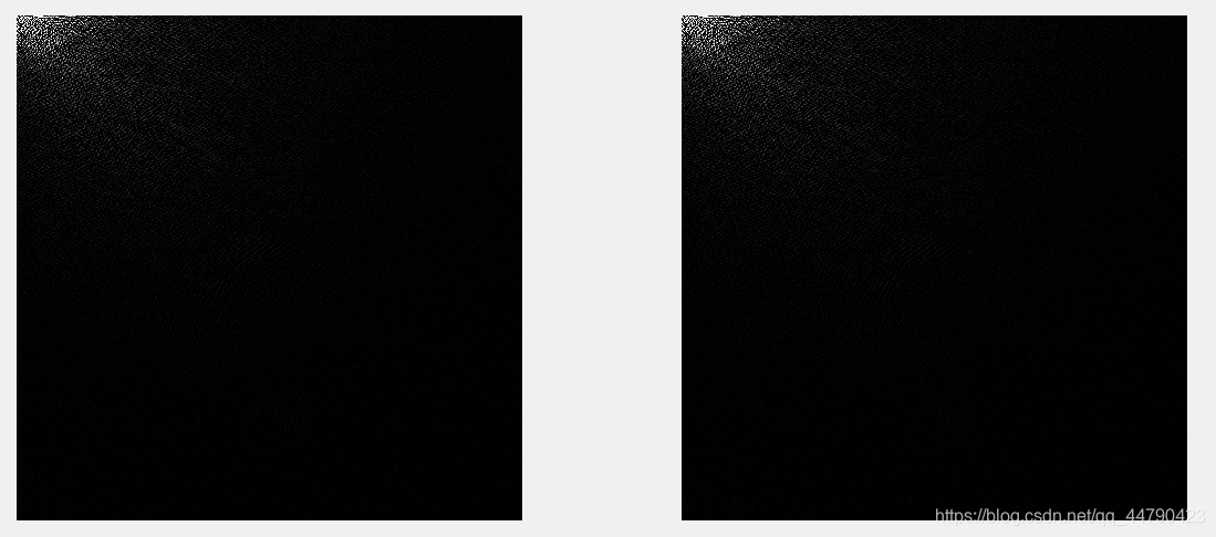
• 图像实现

clear all;
close all;

I = imread('lena_color_512.tif');
I = rgb2gray(I);
I = im2double(I);
s = size(I);
M = s(1);
N = s(2);
P = dctmtx(M);
Q = dctmtx(N);
J = P*I*Q';  %生成矩阵
K = dct2(I);
E = J - K;
find(abs(E) > 0.000001)

figure;
subplot(121), imshow(J);
subplot(122), imshow(K);

左图是采用矩阵来实现的，右图是采用dct2()函数来实现的

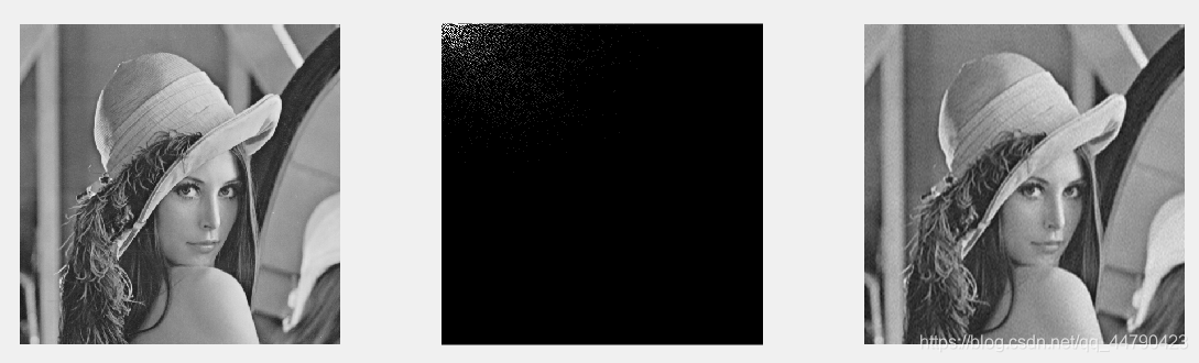
实验idct2

clear all;
close all;

I = imread('lena_color_512.tif');
I = rgb2gray(I);
I = im2double(I);

J = dct2(I);
J(abs(J) < 0.1) = 0;
K = idct2(J);

figure;
subplot(131), imshow(I);
subplot(132), imshow(J);
subplot(133), imshow(K);

下图中左边为原图，中间为变换结果，右边为反变换结果

图像Hadamard变换

clear all;
close all;

I = imread('lena_color_512.tif');
I = rgb2gray(I);
I = im2double(I);
h1 = size(I, 1);
h2 = size(I, 2);
H1 = hadamard(h1);
H2 = hadamard(h2);
J = H1*I*H2/sqrt(h1*h2);


figure;
subplot(121), imshow(I);
subplot(122), imshow(J);

左边为原图，右边为Hadamard的结果

图像Hough变换

Hough变换是 图像处理中从图像中识别几何形状的基本方法之一。由PaulHough于1962年提出，最初只用于二值图像直线检测，后来扩展到任意形状的检测。Hough变换的基本原理在于利用点与线的对偶性，将原始图像空间的给定的曲线通过曲线表达形式变为参数空间的一个点。这样就把原始图像中给定曲线的检测问题转化为寻找参数空间中的峰值问题。

Hough变换根据如下公式：

xcos(θ)+ ysin(θ)= p

---

这里只介绍少部分的变换部分，并不涉及到应用呢，因为能力有限呢~哭泣