MATLAB图像处理之几何变换——平移与旋转

一、图像平移——imtranslate函数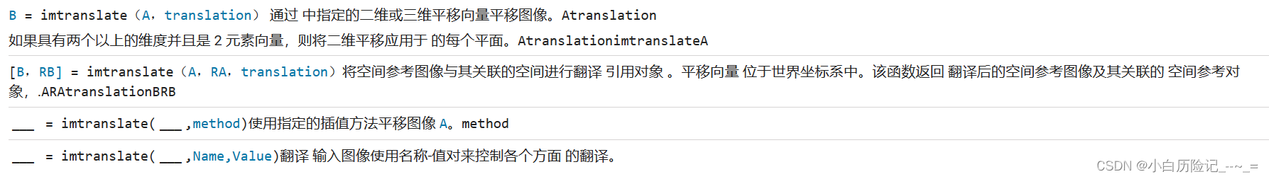

A = imread('cameraman.tif');
V = [50 100];
I = imtranslate(A,V);
figure;
subplot(1,2,1) %创建一个1行2列的坐标区，并在1号位置显示。
imshow(A);
title('原图像')
subplot(1,2,2) %创建一个1行2列的坐标区，并在2号位置显示。
imshow(I);
title("X平移" +V(1)+ ";  Y平移" +V(2)+ "后图像")

可以发现，原图在原坐标基础上向X、Y方向分别平移了50和100个单位。但相应平移的部分也被遮挡了，显然这不符合一些场景的应用需求。
在这里插入图片描述

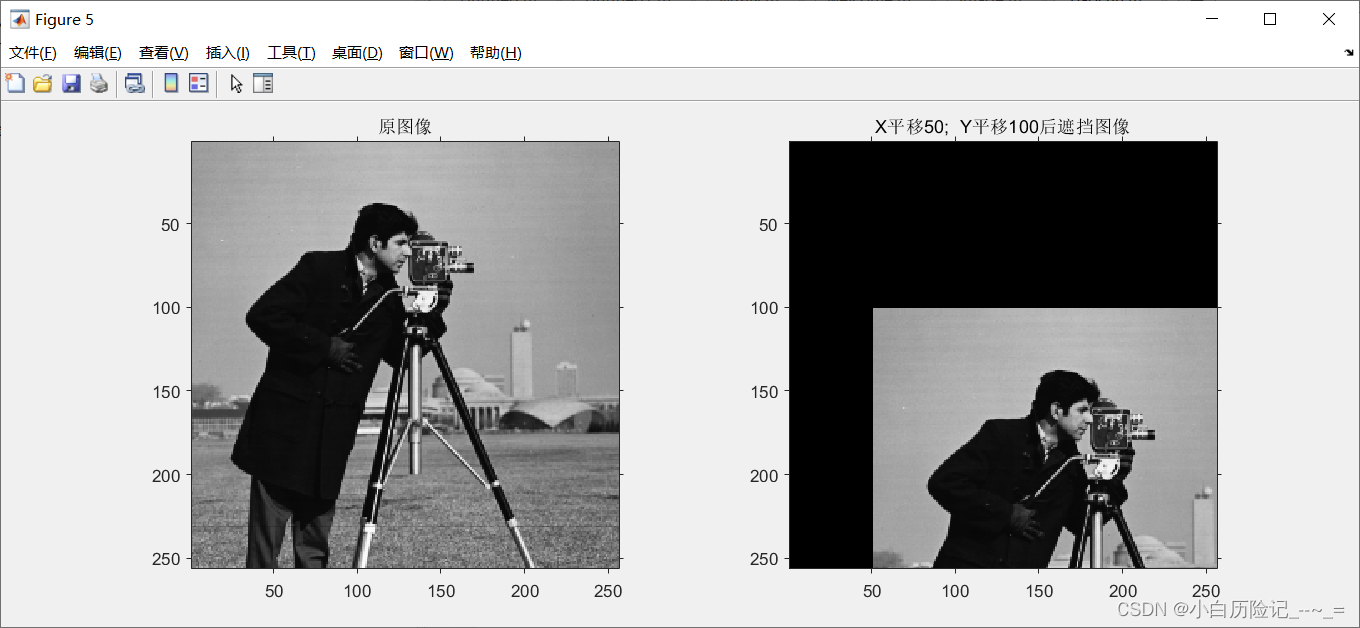
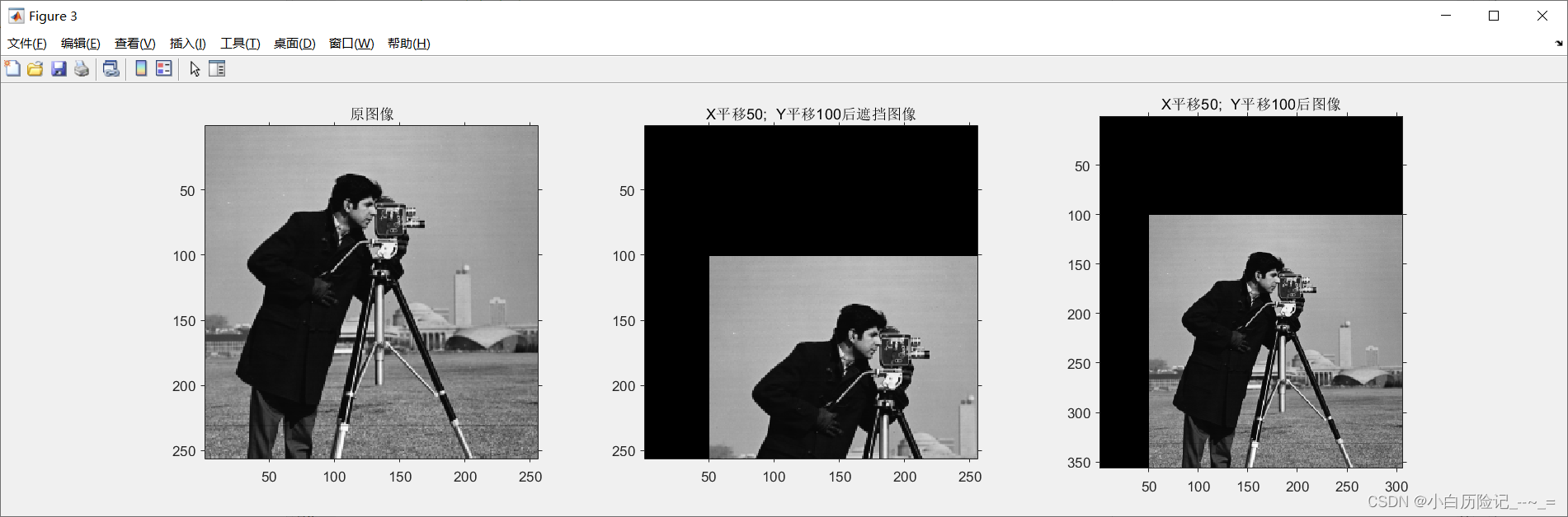
为此，MATLAB还提供了参数设置。在imtranslate函数中设置’OutputView’参数为’full’，即可防止遮挡平移的图像，如下图所示。

A = imread('cameraman.tif');
V = [50 100];
I1 = imtranslate(A,V);
I2 = imtranslate(A,V,'OutputView','full'); %设置参数
figure;
subplot(1,3,1)
imshow(A);
title('原图像')
subplot(1,3,2)
imshow(I1);
title("X平移" +V(1)+ ";  Y平移" +V(2)+ "后遮挡图像")
subplot(1,3,3)
imshow(I2);
title("X平移" +V(1)+ ";  Y平移" +V(2)+ "后图像")

在这里插入图片描述

二、图像旋转——imrotate函数

在这里插入图片描述

MATLAB在进行图像操作时，是将数据存放在数组中，而数组坐标必须为整数，若对图像进行旋转、缩放等操作，计算得到的坐标则不一定为整数，这时候就需要进行插值。通常直接使用 imrotate(I,angle) 就可以了，其默认使用最近邻点插值‘nearest’。也可以使用 imrotate(I,angle，method)，其中method还包括双线性插值 ‘bilinear’和三次卷积插值 ‘bicubic’。

A = imread('cameraman.tif');
B = imrotate(A,30);  % 默认使用最近邻点插值‘nearest’              
C = imrotate(A,30,'bilinear'); % 双线性插值
D = imrotate(A,30,'bicubic'); % 三次卷积插值
figure;
subplot(1,4,1),imshow(A);
title('原图像')
subplot(1,4,2),imshow(B);
title('默认插值')
subplot(1,4,3),imshow(C);
title('双线性插值')
subplot(1,4,4),imshow(D);
title('三次卷积插值')

在这里插入图片描述

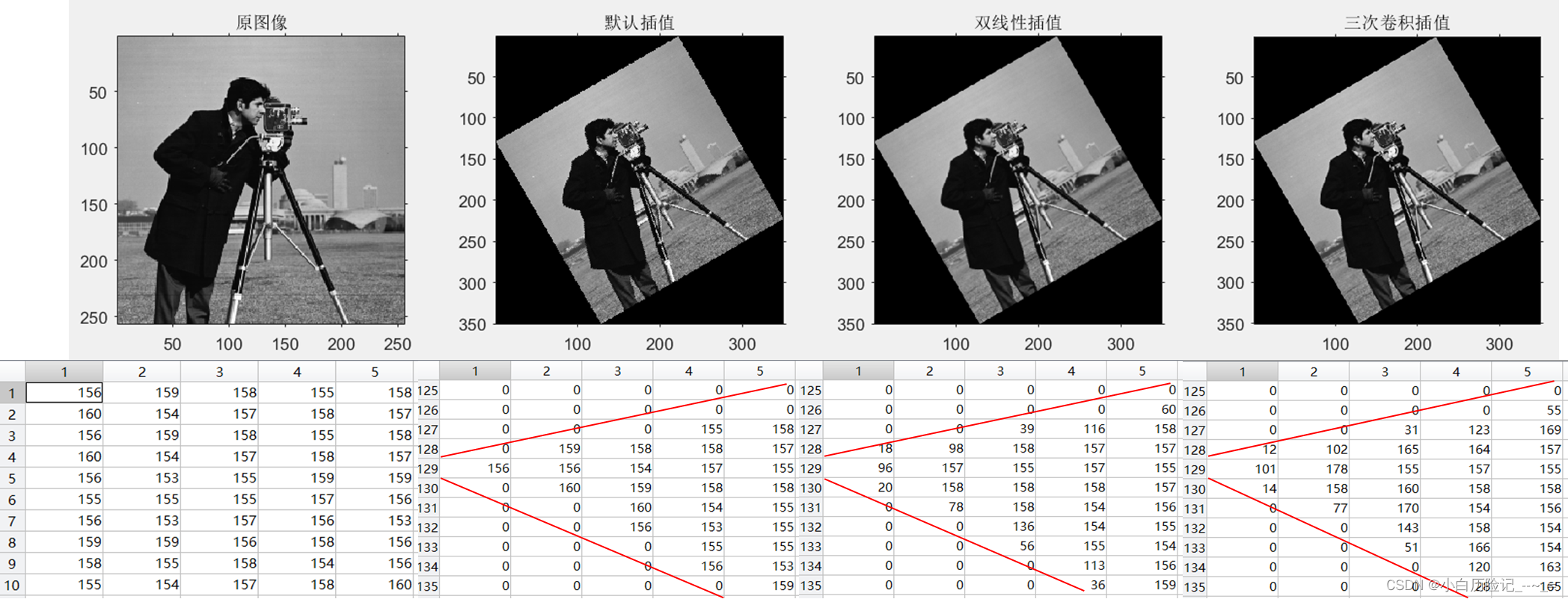
由上图可以发现，经不同插值法旋转后得到的图像肉眼难以看出差别，但对应的数值确有差异，具体选择则需根据实际情况而定。
使用 imrotate(I,angle,method,bbox) 则可以原大小显示。其中bbox — 定义输出图像大小的边界框，包括’loose’ （默认）和 'crop’两参数，'crop’表示使输出图像与输入图像大小相同，裁剪旋转后的图像以适应边界框。

A = imread('cameraman.tif');
B = imrotate(A,30,'crop');                
C = imrotate(A,30,'bilinear','crop');
D = imrotate(A,30,'bicubic','crop');

效果如下，
在这里插入图片描述
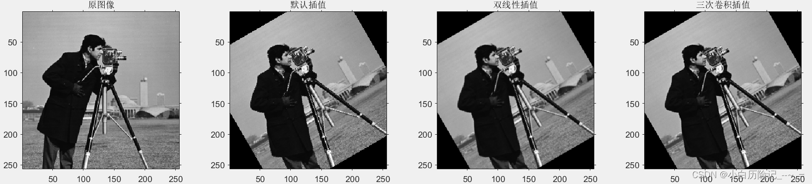
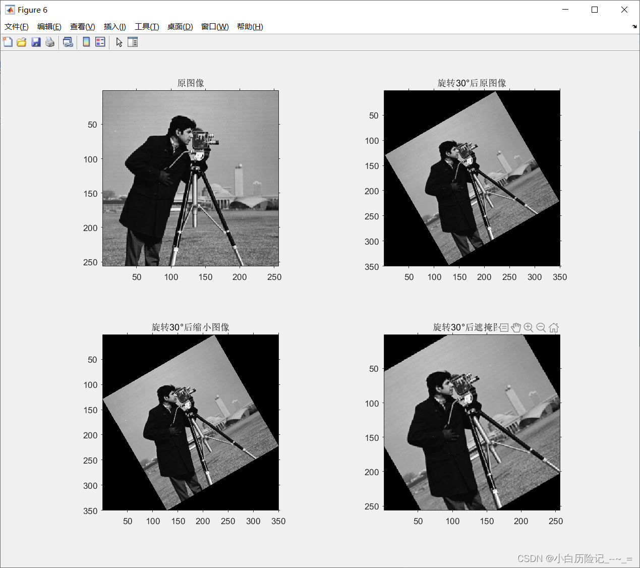
与平移一样，经旋转后的图像虽保留原尺寸大小，但部分被遮掩了，想要原尺寸全图显示则需要自定义函数进行图像计算。

A = imread('cameraman.tif');
% 求出旋转矩阵
rotate = 30;% 旋转角度
theta = rotate / 180 * pi;
R = [cos(theta), -sin(theta); sin(theta), cos(theta)]';
%欧拉角旋转矩阵公式
%利用size函数读取原始图像A尺寸
[m,n,z] = size(A);
length = m;
width = n;
c1 = [length; width] / 2;

% 计算所需背景尺寸
length2 = floor(width*sin(theta)+length*cos(theta))+1;
%floor 向上取整函数，保证图像信息完整
width2 = floor(width*cos(theta)+length*sin(theta))+1;
c2 = [length2; width2] / 2;
% 初始化背景，将旋转后的图像坐标赋给该背景
I = uint8(ones(length2, width2,z));
for k = 1:z
    for i = 1:length2
        for j = 1:width2
            p = [i; j];
            pp = (R*(p-c2)+c1);
            mn = floor(pp);
            ab = pp - mn;
            a = ab(1);
            b = ab(2);
            m = mn(1);
            n = mn(2);
            % 线性插值方法
            if (pp(1) >= 2 && pp(1) <= length-1 && pp(2) >= 2 && pp(2) <= width-1)
                I(i, j, k) = (1-a)*(1-b)*A(m, n, k) + a*(1-b)*A(m+1, n, k)...
                    +(1-a)*b*A(m, n, k)+a*b*A(m, n, k);
            end
        end
    end
end


figure;
subplot(1,2,1),imshow(A);
title('原图像')
subplot(1,2,2)
imshow(I);
title("旋转" +rotate+"°后图像")

以下即为三种旋转方式效果：
在这里插入图片描述