1.Introduction
Gaussian mixture models are a probabilistic model for representing normally distributed subpopulations within an overall population. Mixture models in general don’t require knowing which subpopulation a data point belongs to, allowing the model to learn the subpopulations automatically. Since subpopulation assignment is not known, this constitutes a form of unsupervised learning.GMMs have been used for feature extraction from speech data, and have also been used extensively in object tracking of multiple objects, where the number of mixture components and their means predict object locations at each frame in a video sequence.

One hint that data might follow a mixture model is that the data looks multimodal, i.e. there is more than one “peak” in the distribution of data. Trying to fit a multimodal distribution with a unimodal (one “peak”) model will generally give a poor fit, as shown in the example below. Since many simple distributions are unimodal, an obvious way to model a multimodal distribution would be to assume that it is generated by multiple unimodal distributions. For several theoretical reasons, the most commonly used distribution in modeling real-world unimodal data is the Gaussian distribution. Thus, modeling multimodal data as a mixture of many unimodal Gaussian distributions makes intuitive sense. Furthermore, GMMs maintain many of the theoretical and computational benefits of Gaussian models, making them practical for efficiently modeling very large datasets.
2.Multi-dimensional Model

3.Expectation maximization
Expectation maximization (EM) is a numerical technique for maximum likelihood estimation, and is an iterative algorithm and has the convenient property that the maximum likelihood of the data strictly increases with each subsequent iteration, meaning it is guaranteed to approach a local maximum or saddle point.

Expectation-maximization (EM) algorithm is a general class of algorithm that composed of two sets of parameters θ₁, and θ₂. θ₂ are some un-observed variables, hidden latent factors or missing data. Often, we don’t really care about θ₂ during inference. But if we try to solve the problem, we may find it much easier to break it into two steps and introduce θ₂ as a latent variable. First, we derive θ₂ from the observation and θ₁. Then we optimize θ₁ with θ₂ fixed. We continue the iterations until the solution converges.
In the M-step, we maximize the log-likelihood of the observations w.r.t. θ₁. The log-likelihood ln p(x|θ₁) can be decomposed as the following with the second term being the KL-divergence
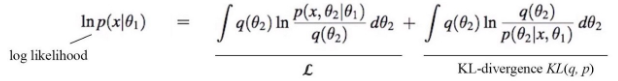
where q(θ₂) can be any distribution.
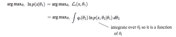
Now, let’s make the R.H.S. as simple as possible so we can optimize it easily. First, let’s pick a choice for q(θ₂). A natural one will be p(θ₂|x, θ₁) — the probability of θ₂ given the observation and our model θ₁. By setting q(θ₂) = p(θ₂|x, θ₁), we get a nice bonus. The KL-divergence term becomes zero. Now our log-likelihood can be simplified to

Since the second term does not change w.r.t. θ₁, we can optimize the R.H.S. term below.
Here is the EM-algorithm:

Gaussian mixture model

猜你喜欢
转载自blog.csdn.net/hahadelaochao/article/details/105626851
今日推荐
周排行