【线性回归算法】{3} ——衡量线性回归算法的指标MSE、RMSE、MAE和R Squared

此处介绍四种线性回归算法的衡量指标。

---

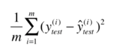
第一种：MSE（均方误差）

第二种：RMSE（均方根误差）

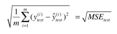
使用RMSE，采用同样的量纲的话，误差背后的意义更加明显。

量纲，又叫作因次，是表示一个物理量由基本量组成的情况。确定若干个基本量后，每个导出量都可以表示为基本量的幂的乘积的形式。引入量纲这一概念可以进行量纲分析，这既是物理学的基础，又有着很多重要应用。——维基百科

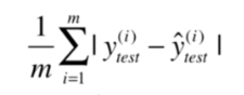
第三种：MAE（平均绝对误差）

---

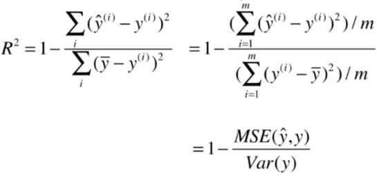
第四种：R Squared（决定系数）

---

首先在PlayML文件夹中写一个model_selection模块，用于分割数据集：

import numpy as np

def train_test_split(X, y, test_ratio=0.2, seed=None):
    if seed:
        np.random.seed(seed)

    shuffled_indexes = np.random.permutation(len(X))

    test_size = int(len(X) * test_ratio)
    test_indexes = shuffled_indexes[:test_size]
    train_indexes = shuffled_indexes[test_size:]

    X_train = X[train_indexes]
    y_train = y[train_indexes]

    X_test = X[test_indexes]
    y_test = y[test_indexes]

    return X_train, X_test, y_train, y_test

---

然后使用线性回归模型拟合波士顿房产数据：

import numpy as np
import matplotlib.pyplot as plt
from sklearn import datasets

boston = datasets.load_boston()

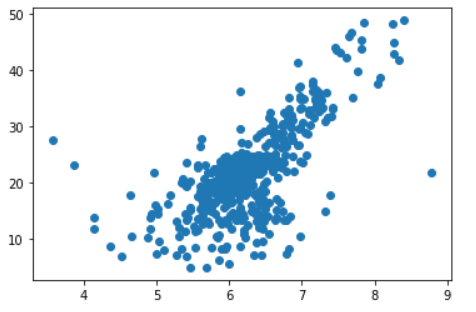
x = boston.data[:,5] # 只取出第5列（房间数量这一特征）
y = boston.target

x = x[y < 50.0] # 剔除超过50的点（因为有可能有超过50的，但是在图中只显示50）
y = y[y < 50.0]

plt.scatter(x, y)
plt.show()

Output：

---

from playML.model_selection import train_test_split # 分割数据集
from playML.SimpleLinearRegression import SimpleLinearRegression2

x_train, x_test, y_train, y_test = train_test_split(x, y, seed=666)

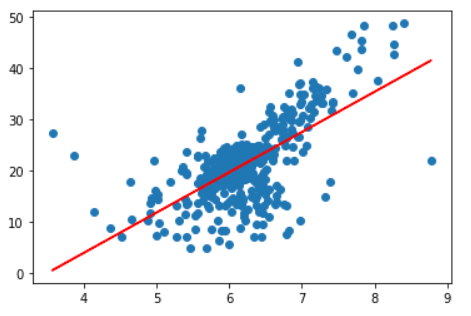
reg = SimpleLinearRegression2()
reg.fit(x_train, y_train)

plt.scatter(x_train, y_train)
plt.plot(x_train, reg.predict(x_train), color='r')
plt.show()

Output：

---

接下来使用上述指标衡量我们的模型：

y_predict = reg.predict(x_test)

---

MSE（均方误差）：

mse_test = np.sum((y_predict - y_test)**2) / len(y_test)
print(mse_test)

Output：

---

RMSE（均方根误差）：

from math import sqrt

rmse_test = sqrt(mse_test)
print(rmse_test)

---

MAE（平均绝对误差）：

mae_test = np.sum(np.absolute(y_predict - y_test)) / len(y_test)
print(mae_test)

---

R Squared（决定系数）：

print(1 - mean_squared_error(y_test, y_predict) / np.var(y_test))

---

计算上面指标的算法可以封装成一个模块

---

参考资料：bobo老师机器学习教程