[CS231n Assignment 2] 全连接神经网络(Fully-connected Neural Network)

作业介绍

• 作业主页：Assignment 2
• 作业目的：之前我们已经实现过一个双层的神经网络了，但是，它的所有函数被放置在一个文件中。对于，简单的神经网络，这种做法或许比较简便，但是当我们需要更大、更深的神经网络的时候，这种写法可能就不是那么高效。所以，本次作业，我们需要学会如何对神经网络进行 分层设计 以及 模块化，在不同的文件中实现我们不同的模块，然后将它们 整合 成最终的网络。
• 官方示例代码： Assignment 2 code
• 作业源文件 FullyConnectedNets.ipynb

1.Fully-Connected Neural Nets 架构

在本次作业中，我们将模块化的实现我们的全连接神经网络，每一层网络，我们将实现前向传播forward() 和反向传播 backward()。

• 其中，forward()接收输入和权重以及必要的其它参数，然后返回一个输出，以及存储我们在反向传播过程中需要的变量，即类似于：

def layer_forward(x, w):
  """ Receive inputs x and weights w """
  # Do some computations ...
  z = # ... some intermediate value
  # Do some more computations ...
  out = # the output

  cache = (x, w, z, out) # Values we need to compute gradients

  return out, cache

• 而反向传播过程backward()将接收上流梯度以及之前存储的变量，然后返回输入以及权重的梯度：

def layer_backward(dout, cache):
  """
  Receive dout (derivative of loss with respect to outputs) and cache,
  and compute derivative with respect to inputs.
  """
  # Unpack cache values
  x, w, z, out = cache

  # Use values in cache to compute derivatives
  dx = # Derivative of loss with respect to x
  dw = # Derivative of loss with respect to w

  return dx, dw

2. 初始化作业环境

• 下载数据集
• 安装必要的包

• 注意：gnureadline==6.3.3 在windows下不支持，直接不安装就行；其它也并不都是必须的，可选择性安装，但是要有Numpy、Cython、Future等。

cd assignment2
pip install -r requirements.txt

• 编译Cython扩展：因为卷积神经网络需要一些高效的操作，所以官方已经用Cython实现了必要的操作，例如im2col.py。我们要做的就是先编译这个文件，即：在cs231n目录下，运行setup.py

python setup.py build_ext --inplace

• 初始化Jupyter notebook环境

# As usual, a bit of setup
from __future__ import print_function
import time
import numpy as np
import matplotlib.pyplot as plt
from cs231n.classifiers.fc_net import *
from cs231n.data_utils import get_CIFAR10_data
from cs231n.gradient_check import eval_numerical_gradient, eval_numerical_gradient_array
from cs231n.solver import Solver

%matplotlib inline
plt.rcParams['figure.figsize'] = (10.0, 8.0) # set default size of plots
plt.rcParams['image.interpolation'] = 'nearest'
plt.rcParams['image.cmap'] = 'gray'

# for auto-reloading external modules
# see http://stackoverflow.com/questions/1907993/autoreload-of-modules-in-ipython
%load_ext autoreload
%autoreload 2

def rel_error(x, y):
  """ returns relative error """
  return np.max(np.abs(x - y) / (np.maximum(1e-8, np.abs(x) + np.abs(y))))

• 加载数据：

# Load the (preprocessed) CIFAR10 data.

data = get_CIFAR10_data()
for k, v in list(data.items()):
  print(('%s: ' % k, v.shape))

('X_val: ', (1000, 3, 32, 32))
('y_test: ', (1000,))
('y_train: ', (49000,))
('X_test: ', (1000, 3, 32, 32))
('X_train: ', (49000, 3, 32, 32))
('y_val: ', (1000,))

3. 实现全连接层(Affine Layer)

3.1 前向传播

• Open the file cs231n/layers.py and implement the affine_forward function.

def affine_forward(x, w, b):
    """
    Computes the forward pass for an affine (fully-connected) layer.

    The input x has shape (N, d_1, ..., d_k) and contains a minibatch of N
    examples, where each example x[i] has shape (d_1, ..., d_k). We will
    reshape each input into a vector of dimension D = d_1 * ... * d_k, and
    then transform it to an output vector of dimension M.

    Inputs:
    - x: A numpy array containing input data, of shape (N, d_1, ..., d_k)
    - w: A numpy array of weights, of shape (D, M)
    - b: A numpy array of biases, of shape (M,)

    Returns a tuple of:
    - out: output, of shape (N, M)
    - cache: (x, w, b)
    """
    out = None
    # reshape the input into rows.
    x = x.reshape(x.shape[0],-1) # [N , D]
    out = np.dot(x,w) + b # [N , M]
    cache = (x, w, b)
    return out, cache

3.2 反向传播

• Now implement the affine_backward function and test your implementation using numeric gradient checking.

def affine_backward(dout, cache):
    """
    Computes the backward pass for an affine layer.

    Inputs:
    - dout: Upstream derivative, of shape (N, M)
    - cache: Tuple of:
      - x: Input data, of shape (N, d_1, ... d_k)
      - w: Weights, of shape (D, M)
      - b: Biases, of shape (M,)

    Returns a tuple of:
    - dx: Gradient with respect to x, of shape (N, d1, ..., d_k)
    - dw: Gradient with respect to w, of shape (D, M)
    - db: Gradient with respect to b, of shape (M,)
    """
    x, w, b = cache
    x_rows = x.reshape(x.shape[0],-1)
    d_xrows = np.dot(dout,w.T)
    dx = d_xrows.reshape(x.shape)
    dw = np.dot(x_rows.T, dout)
    # 注意，这里的db没有对行取平均
    db = np.sum(dout, axis=0)
    return dx, dw, db

4. ReLU激活函数

def relu_forward(x):
    """
    Computes the forward pass for a layer of rectified linear units (ReLUs).

    Input:
    - x: Inputs, of any shape

    Returns a tuple of:
    - out: Output, of the same shape as x
    - cache: x
    """
    out = np.maximum(0,x)
    cache = x
    return out, cache


def relu_backward(dout, cache):
    """
    Computes the backward pass for a layer of rectified linear units (ReLUs).

    Input:
    - dout: Upstream derivatives, of any shape
    - cache: Input x, of same shape as dout

    Returns:
    - dx: Gradient with respect to x
    """
    dx, x = None, cache
    dx = (x > 0) * dout
    return dx

5. “Sandwich” layers

我们经常会在FC层后面添加ReLU激活函数，请在cs231n/layer_utils.py.中实现该组合。也算是简单的模型设计组合练习。

def affine_relu_forward(x, w, b):
    """
    Convenience layer that perorms an affine transform followed by a ReLU

    Inputs:
    - x: Input to the affine layer
    - w, b: Weights for the affine layer

    Returns a tuple of:
    - out: Output from the ReLU
    - cache: Object to give to the backward pass
    """
    a, fc_cache = affine_forward(x, w, b)
    out, relu_cache = relu_forward(a)
    cache = (fc_cache, relu_cache)
    return out, cache


def affine_relu_backward(dout, cache):
    """
    Backward pass for the affine-relu convenience layer
    """
    fc_cache, relu_cache = cache
    da = relu_backward(dout, relu_cache)
    dx, dw, db = affine_backward(da, fc_cache)
    return dx, dw, db

6. 损失层(Loss Layer)

• You implemented these loss functions in the last assignment, so we’ll give them to you for free here. You should still make sure you understand how they work by looking at the implementations in cs231n/layers.py.

• 居然还有这种好事，不过大家可以和前面自己实现的比较一下。

def svm_loss(x, y):
    """
    Computes the loss and gradient using for multiclass SVM classification.

    Inputs:
    - x: Input data, of shape (N, C) where x[i, j] is the score for the jth
      class for the ith input.
    - y: Vector of labels, of shape (N,) where y[i] is the label for x[i] and
      0 <= y[i] < C

    Returns a tuple of:
    - loss: Scalar giving the loss
    - dx: Gradient of the loss with respect to x
    """
    N = x.shape[0]
    correct_class_scores = x[np.arange(N), y]
    margins = np.maximum(0, x - correct_class_scores[:, np.newaxis] + 1.0)
    margins[np.arange(N), y] = 0
    loss = np.sum(margins) / N
    num_pos = np.sum(margins > 0, axis=1)
    dx = np.zeros_like(x)
    dx[margins > 0] = 1
    dx[np.arange(N), y] -= num_pos
    dx /= N
    return loss, dx


def softmax_loss(x, y):
    """
    Computes the loss and gradient for softmax classification.

    Inputs:
    - x: Input data, of shape (N, C) where x[i, j] is the score for the jth
      class for the ith input.
    - y: Vector of labels, of shape (N,) where y[i] is the label for x[i] and
      0 <= y[i] < C

    Returns a tuple of:
    - loss: Scalar giving the loss
    - dx: Gradient of the loss with respect to x
    """
    shifted_logits = x - np.max(x, axis=1, keepdims=True)
    Z = np.sum(np.exp(shifted_logits), axis=1, keepdims=True)
    log_probs = shifted_logits - np.log(Z)
    probs = np.exp(log_probs)
    N = x.shape[0]
    loss = -np.sum(log_probs[np.arange(N), y]) / N
    dx = probs.copy()
    dx[np.arange(N), y] -= 1
    dx /= N
    return loss, dx

• 损失层主要放在最后，所以没有保存中间变量，直接返回损失和回传梯度。

7. 两层神经网络（Two-layer network）

• 用我们之前实现的层来搭建一个二层全连接神经网络

• Open the file cs231n/classifiers/fc_net.py and complete the implementation of the TwoLayerNet class. This class will serve as a model for the other networks you will implement in this assignment, so read through it to make sure you understand the API. You can run the cell below to test your implementation.

• AFFINE->RELU->AFFINE->Softmax
  同时，这个Module不进行具体的梯度下降优化，它之后会与一个Solver交互来进行具体的梯度下降。

• 而且，它需要学习的参数存储在一个字典self.params中

class TwoLayerNet(object):
    """
    A two-layer fully-connected neural network with ReLU nonlinearity and
    softmax loss that uses a modular layer design. We assume an input dimension
    of D, a hidden dimension of H, and perform classification over C classes.

    The architecure should be affine - relu - affine - softmax.

    Note that this class does not implement gradient descent; instead, it
    will interact with a separate Solver object that is responsible for running
    optimization.

    The learnable parameters of the model are stored in the dictionary
    self.params that maps parameter names to numpy arrays.
    """

    def __init__(self, input_dim=3*32*32, hidden_dim=100, num_classes=10,
                 weight_scale=1e-3, reg=0.0):
        """
        Initialize a new network.

        Inputs:
        - input_dim: An integer giving the size of the input
        - hidden_dim: An integer giving the size of the hidden layer
        - num_classes: An integer giving the number of classes to classify
        - weight_scale: Scalar giving the standard deviation for random
          initialization of the weights.
        - reg: Scalar giving L2 regularization strength.
        """
        self.params = {}
        self.reg = reg

        # TODO: Initialize the weights and biases of the two-layer net. Weights    #
        # should be initialized from a Gaussian centered at 0.0 with               #
        # standard deviation equal to weight_scale, and biases should be           #
        # initialized to zero.
        self.params["W1"] = np.random.randn(input_dim,hidden_dim) * weight_scale
        self.params["b1"] = np.zeros_like(hidden_dim)
        self.params["W2"] = np.random.randn(hidden_dim,num_classes) * weight_scale
        self.params["b2"] = np.zeros_like(num_classes)
    def loss(self, X, y=None):
        """
        Compute loss and gradient for a minibatch of data.

        Inputs:
        - X: Array of input data of shape (N, d_1, ..., d_k)
        - y: Array of labels, of shape (N,). y[i] gives the label for X[i].

        Returns:
        If y is None, then run a test-time forward pass of the model and return:
        - scores: Array of shape (N, C) giving classification scores, where
          scores[i, c] is the classification score for X[i] and class c.

        If y is not None, then run a training-time forward and backward pass and
        return a tuple of:
        - loss: Scalar value giving the loss
        - grads: Dictionary with the same keys as self.params, mapping parameter
          names to gradients of the loss with respect to those parameters.
        """
        ############################################################################
        # TODO: Implement the forward pass for the two-layer net, computing the#
        # class scores for X and storing them in the scores variable.              #
        ############################################################################
        H , cache_layer1 = affine_relu_forward(X,self.params["W1"],self.params["b1"])
        scores , cache_layer2 = affine_forward(H, self.params["W2"], self.params["b2"])
        # If y is None then we are in test mode so just return scores
        if y is None:
            return scores

        loss, grads = 0, {}
        ############################################################################
        # TODO: Implement the backward pass for the two-layer net. Store the loss  #
        # in the loss variable and gradients in the grads dictionary. Compute data #
        # loss using softmax, and make sure that grads[k] holds the gradients for  #
        # self.params[k]. Don't forget to add L2 regularization!                   #
        #                                                                          #
        # NOTE: To ensure that your implementation matches ours and you pass the   #
        # automated tests, make sure that your L2 regularization includes a factor #
        # of 0.5 to simplify the expression for the gradient.                      #
        ############################################################################
        loss, dS = softmax_loss(scores,y)
        loss += 0.5 * self.reg * np.sum(self.params["W1"] * self.params["W1"])
        loss += 0.5 * self.reg * np.sum(self.params["W2"] * self.params["W2"]) # 添加正则项

        dH , dW2 , grads["b2"] = affine_backward(dS,cache_layer2)
        dx, dW1,grads["b1"] = affine_relu_backward(dH , cache_layer1)

        grads["W1"] = dW1 + self.reg * self.params["W1"]
        grads["W2"] = dW2 + self.reg * self.params["W2"] # 正则项损失
        return loss, grads

• 易错点：最后的损失要加上正则损失，且正则损失要乘以一个正则强度；同时，权重的梯度需要加上一个正则梯度

8. 优化器（Solver）

• for this assignment we have split the logic for training models into a separate class.
• Open the file cs231n/solver.py and read through it to familiarize yourself with the API. After doing so, use a Solver instance to train a TwoLayerNet that achieves at least 50% accuracy on the validation set.

8.1 Solver剖析

这个抽象分离得很好，前面的模型API负责接收数据，计算损失和梯度，这里的Solver复杂将数据组织进行输入，以及返回梯度并使用给定的优化方法更新梯度。这样，我们能用相同的Solver抽象来优化不同的模型，即 这是所有模型公共的部分，所以可以单独抽象出来。

• __init__(self, model, data, **kwargs)
  初始化方法接收我们的模型实例，以及数据输入，同时可选参数包括我们的训练参数，以及优化方法的参数（因为有些优化方法是有参数的，最基本的就是学习率）

参数名	具体含义
update_rule：string	优化方法名字，会传给optim.py
optim_config：dict	存储优化器的参数，例如学习率
lr_decay	每个epoch后学习率的衰减尺度
batch_size	每个batch样本数目
num_epochs	总的epoch数目
print_every	打印训练损失的迭代(iterations)间隔
verbose	是否打印训练的状态
num_train_samples	每个epoch之后拿来计算精度的训练样本数
num_val_samples	每个epoch之后拿来计算精度的验证集样本数
checkpoint_name	保存的模型检查点名字，需要包括模型参数和我们的配置参数，便于下次恢复训练

• 然后init()方法暂存这些输入的参数

    def __init__(self, model, data, **kwargs):
        """
        Construct a new Solver instance.
        """
        self.model = model
        self.X_train = data['X_train']
        self.y_train = data['y_train']
        self.X_val = data['X_val']
        self.y_val = data['y_val']

        # Unpack keyword arguments
        self.update_rule = kwargs.pop('update_rule', 'sgd')
        self.optim_config = kwargs.pop('optim_config', {})
        self.lr_decay = kwargs.pop('lr_decay', 1.0)
        self.batch_size = kwargs.pop('batch_size', 100)
        self.num_epochs = kwargs.pop('num_epochs', 10)
        self.num_train_samples = kwargs.pop('num_train_samples', 1000)
        self.num_val_samples = kwargs.pop('num_val_samples', None)

        self.checkpoint_name = kwargs.pop('checkpoint_name', None)
        self.print_every = kwargs.pop('print_every', 10)
        self.verbose = kwargs.pop('verbose', True)

        # Throw an error if there are extra keyword arguments
        if len(kwargs) > 0:
            extra = ', '.join('"%s"' % k for k in list(kwargs.keys()))
            raise ValueError('Unrecognized arguments %s' % extra)

        # Make sure the update rule exists, then replace the string
        # name with the actual function
        if not hasattr(optim, self.update_rule):
            raise ValueError('Invalid update_rule "%s"' % self.update_rule)
        # now, it's a function
        self.update_rule = getattr(optim, self.update_rule)

        self._reset()

• 然后init()方法调用了_reset()方法，其初始化了一些训练时的状态参数，并且给模型中的每一个参数都设置了优化规则的参数，方便之后传模型参数+优化参数给optim来进行权重更新

    def _reset(self):
        """
        Set up some book-keeping variables for optimization. Don't call this
        manually.
        """
        # Set up some variables for book-keeping
        self.epoch = 0
        self.best_val_acc = 0
        self.best_params = {}
        self.loss_history = []
        self.train_acc_history = []
        self.val_acc_history = []

        # Make a deep copy of the optim_config for each parameter
        self.optim_configs = {}
        for p in self.model.params:
            d = {k: v for k, v in self.optim_config.items()}
            self.optim_configs[p] = d

• 然后是_step()方法，其使用一个batchsize的数据对权重参数进行更新

    def _step(self):
        """
        Make a single gradient update. This is called by train() and should not
        be called manually.
        """
        # Make a minibatch of training data
        num_train = self.X_train.shape[0]
        batch_mask = np.random.choice(num_train, self.batch_size)
        X_batch = self.X_train[batch_mask]
        y_batch = self.y_train[batch_mask]

        # Compute loss and gradient
        loss, grads = self.model.loss(X_batch, y_batch)
        self.loss_history.append(loss)

        # Perform a parameter update
        for p, w in self.model.params.items():
            dw = grads[p]
            config = self.optim_configs[p]
            next_w, next_config = self.update_rule(w, dw, config)
            self.model.params[p] = next_w
            self.optim_configs[p] = next_config

• _save_checkpoint()函数保存当前模型参数以及配置参数

        if self.checkpoint_name is None: return
        checkpoint = {
          'model': self.model,
          'update_rule': self.update_rule,
          'lr_decay': self.lr_decay,
          'optim_config': self.optim_config,
          'batch_size': self.batch_size,
          'num_train_samples': self.num_train_samples,
          'num_val_samples': self.num_val_samples,
          'epoch': self.epoch,
          'loss_history': self.loss_history,
          'train_acc_history': self.train_acc_history,
          'val_acc_history': self.val_acc_history,
        }
        filename = '%s_epoch_%d.pkl' % (self.checkpoint_name, self.epoch)
        if self.verbose:
            print('Saving checkpoint to "%s"' % filename)
        with open(filename, 'wb') as f:
            pickle.dump(checkpoint, f)

• check_accuracy(X, y, num_samples=None, batch_size=100) 在每个epoch之后，从X中抽取样本num_samples计算准确度，而且为了防止数据量过大，一次只取一个batchsize来计算

    def check_accuracy(self, X, y, num_samples=None, batch_size=100):
        """
        Check accuracy of the model on the provided data.

        Inputs:
        - X: Array of data, of shape (N, d_1, ..., d_k)
        - y: Array of labels, of shape (N,)
        - num_samples: If not None, subsample the data and only test the model
          on num_samples datapoints.
        - batch_size: Split X and y into batches of this size to avoid using
          too much memory.

        Returns:
        - acc: Scalar giving the fraction of instances that were correctly
          classified by the model.
        """
        # Maybe subsample the data
        N = X.shape[0]
        if num_samples is not None and N > num_samples:
            mask = np.random.choice(N, num_samples)
            N = num_samples
            X = X[mask]
            y = y[mask]

        # Compute predictions in batches
        num_batches = N // batch_size
        if N % batch_size != 0:
            num_batches += 1
        y_pred = []
        for i in range(num_batches):
            start = i * batch_size
            end = (i + 1) * batch_size
            scores = self.model.loss(X[start:end])
            y_pred.append(np.argmax(scores, axis=1))
        y_pred = np.hstack(y_pred)
        acc = np.mean(y_pred == y)

• 最后就是我们外部真正可以调用的train()方法了，首先，其根据我们的batchsize来计算我么进行一个epoch需要多少次迭代iteration，然后计算总的迭代数。每个epoch之后，我们都衰减学习率learning_rate，且每个epoch之后，我们都计算一下训练集和验证集的精确度。

    def train(self):
        """
        Run optimization to train the model.
        """
        num_train = self.X_train.shape[0]
        iterations_per_epoch = max(num_train // self.batch_size, 1)
        num_iterations = self.num_epochs * iterations_per_epoch

        for t in range(num_iterations):
            self._step()

            # Maybe print training loss
            if self.verbose and t % self.print_every == 0:
                print('(Iteration %d / %d) loss: %f' % (
                       t + 1, num_iterations, self.loss_history[-1]))

            # At the end of every epoch, increment the epoch counter and decay
            # the learning rate.
            epoch_end = (t + 1) % iterations_per_epoch == 0
            if epoch_end:
                self.epoch += 1
                for k in self.optim_configs:
                    self.optim_configs[k]['learning_rate'] *= self.lr_decay

            # Check train and val accuracy on the first iteration, the last
            # iteration, and at the end of each epoch.
            first_it = (t == 0)
            last_it = (t == num_iterations - 1)
            if first_it or last_it or epoch_end:
                train_acc = self.check_accuracy(self.X_train, self.y_train,
                    num_samples=self.num_train_samples)
                val_acc = self.check_accuracy(self.X_val, self.y_val,
                    num_samples=self.num_val_samples)
                self.train_acc_history.append(train_acc)
                self.val_acc_history.append(val_acc)
                self._save_checkpoint()

                if self.verbose:
                    print('(Epoch %d / %d) train acc: %f; val_acc: %f' % (
                           self.epoch, self.num_epochs, train_acc, val_acc))

                # Keep track of the best model
                if val_acc > self.best_val_acc:
                    self.best_val_acc = val_acc
                    self.best_params = {}
                    for k, v in self.model.params.items():
                        self.best_params[k] = v.copy()

        # At the end of training swap the best params into the model
        self.model.params = self.best_params

8.2 实际训练

• 设置好优化器的参数，我们实际训练，注意我刚开始在训练的时候使用的是默认的学习率1e-2，发现权重更新太大，很快损失就增长到 nan了

model = TwoLayerNet()

##############################################################################
# TODO: Use a Solver instance to train a TwoLayerNet that achieves at least  #
# 50% accuracy on the validation set.                                        #
##############################################################################
solver = Solver(model,data,
                num_epochs = 30,
                update_rule = 'sgd',
                optim_config = {
                    'learning_rate': 1e-3
                },
                lr_decay = 0.95,
                batch_size = 128,
                print_every = 100
               )
solver.train()

可视化训练过程

plt.subplot(2, 1, 1)
plt.title('Training loss')
plt.plot(solver.loss_history, 'o')
plt.xlabel('Iteration')

plt.subplot(2, 1, 2)
plt.title('Accuracy')
plt.plot(solver.train_acc_history, '-o', label='train')
plt.plot(solver.val_acc_history, '-o', label='val')
plt.plot([0.5] * len(solver.val_acc_history), 'k--')
plt.xlabel('Epoch')
plt.legend(loc='lower right')
plt.gcf().set_size_inches(15, 12)
plt.show()

9. 多层神经网络（Multilayer network）

• 这次我们实现一个含有任意隐藏层的全连接神经网络
• Read through the FullyConnectedNet class in the file cs231n/classifiers/fc_net.py.

# 第一步可以先不实现BN和Dropout
class FullyConnectedNet(object):
    """
    A fully-connected neural network with an arbitrary number of hidden layers,
    ReLU nonlinearities, and a softmax loss function. This will also implement
    dropout and batch/layer normalization as options. For a network with L layers,
    the architecture will be

    {affine - [batch/layer norm] - relu - [dropout]} x (L - 1) - affine - softmax

    where batch/layer normalization and dropout are optional, and the {...} block is
    repeated L - 1 times.

    Similar to the TwoLayerNet above, learnable parameters are stored in the
    self.params dictionary and will be learned using the Solver class.
    """

    def __init__(self, hidden_dims, input_dim=3*32*32, num_classes=10,
                 dropout=1, normalization=None, reg=0.0,
                 weight_scale=1e-2, dtype=np.float32, seed=None):
        
        self.normalization = normalization
        self.use_dropout = dropout != 1
        self.reg = reg
        self.num_layers = 1 + len(hidden_dims)
        self.dtype = dtype
        self.params = {}
        
        input_size = input_dim
        for i in range(len(hidden_dims)):
            output_size = hidden_dims[i]
            self.params['W' + str(i+1)] = np.random.randn(input_size,output_size) * weight_scale
            self.params['b' + str(i+1)] = np.zeros(output_size)
            if not self.normalization is None:
                self.params['gamma' + str(i+1)] = np.ones(output_size)
                self.params['beta' + str(i+1)] = np.zeros(output_size)
            input_size = output_size # 下一层的输入
        # 输出层，没有BN操作
        self.params['W' + str(self.num_layers)] = np.random.randn(input_size,num_classes) * weight_scale
        self.params['b' + str(self.num_layers)] = np.zeros(num_classes)
        # When using dropout we need to pass a dropout_param dictionary to each
        # dropout layer so that the layer knows the dropout probability and the mode
        # (train / test). You can pass the same dropout_param to each dropout layer.
        self.dropout_param = {}
        if self.use_dropout:
            self.dropout_param = {'mode': 'train', 'p': dropout}
            if seed is not None:
                self.dropout_param['seed'] = seed

        self.bn_params = []
        if self.normalization=='batchnorm':
            self.bn_params = [{'mode': 'train'} for i in range(self.num_layers - 1)]
        if self.normalization=='layernorm':
            self.bn_params = [{} for i in range(self.num_layers - 1)]

        # Cast all parameters to the correct datatype
        for k, v in self.params.items():
            self.params[k] = v.astype(dtype)


    def loss(self, X, y=None):
        """
        Compute loss and gradient for the fully-connected net.

        Input / output: Same as TwoLayerNet above.
        """
        X = X.astype(self.dtype)
        mode = 'test' if y is None else 'train'

        # Set train/test mode for batchnorm params and dropout param since they
        # behave differently during training and testing.
        if self.use_dropout:
            self.dropout_param['mode'] = mode
        if self.normalization=='batchnorm':
            for bn_param in self.bn_params:
                bn_param['mode'] = mode
        
        cache = {} # 需要存储反向传播需要的参数
        hidden = X
        for i in range(self.num_layers - 1):
            if self.normalization :
                pass
            else:
                hidden , cache[i+1] = affine_relu_forward(hidden,self.params['W' + str(i+1)],
                                                          self.params['b' + str(i+1)])
            if self.use_dropout:
                pass
        # 最后一层不用激活
        scores, cache[self.num_layers] = affine_forward(hidden , self.params['W' + str(self.num_layers)],
                                                       self.params['b' + str(self.num_layers)])

        # If test mode return early
        if mode == 'test':
            return scores
            
        loss, grads = 0.0, {}
        loss, dS = softmax_loss(scores , y)
        # 最后一层没有relu激活
        dhidden, grads['W' + str(self.num_layers)], grads['b' + str(self.num_layers)] \
            = affine_backward(dS,cache[self.num_layers])
        loss += 0.5 * self.reg * np.sum(self.params['W' + str(self.num_layers)] * self.params['W' + str(self.num_layers)])
        grads['W' + str(self.num_layers)] += self.reg * self.params['W' + str(self.num_layers)]

        for i in range(self.num_layers - 1, 0, -1):
            loss += 0.5 * self.reg * np.sum(self.params["W" + str(i)] * self.params["W" + str(i)])
            # 倒着求梯度
            if self.use_dropout:
                pass
            if self.normalization:
                pass
            else:
                dhidden, dw, db = affine_relu_backward(dhidden, cache[i])
            grads['W' + str(i)] = dw + self.reg * self.params['W' + str(i)]
            grads['b' + str(i)] = db
        return loss, grads

• 然后我们试着训练来过拟合一个小的数据集（来检验一个完整性）
  不过这个部分有点坑，只调学习率和初始化因子来让20个epoch之内完全过拟合训练集，大家看着调把，实在不行，先随机搜索一下，看哪个学习率区间内能做到过拟合。而且，发现 权重初始化也特别重要，相同的学习率，有些权重初始化就直接崩掉了。

from random import uniform
for i in range(10):
	lr = 10**unifor(-1,-3)
	weight_scale = 10**uniform(-1,-4)
	test_it()

10. 更新规则（Update-rule）

之前，我们训练神经网络都是使用了朴素的sgd算法，这一节，我们会实现其它更新规则来更新我们的参数，它们被定义在optim.py

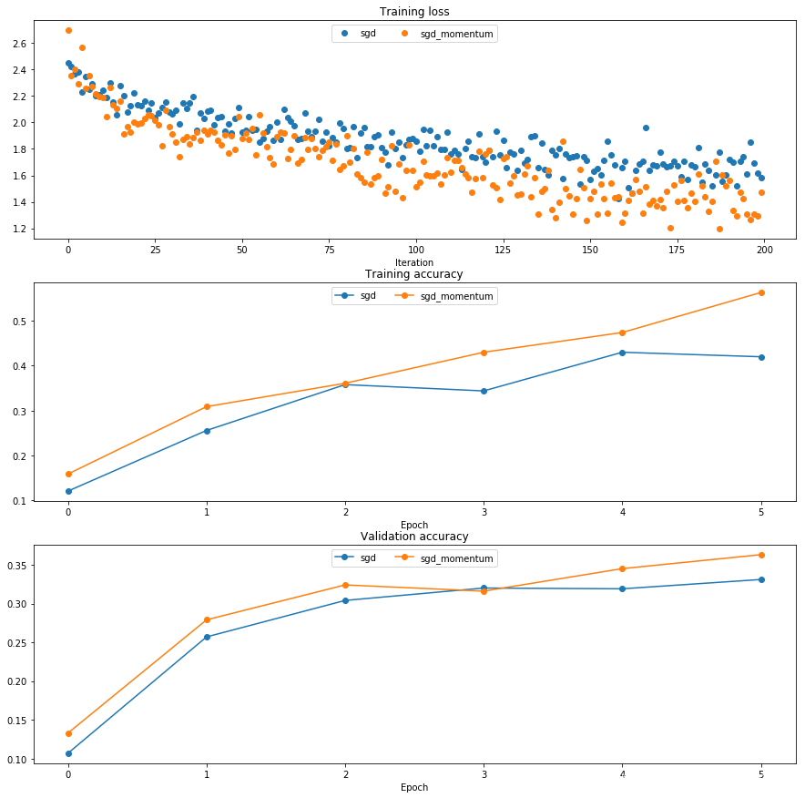
10.1 SGD+Momentum

• 梯度影响当前速度，而不直接影响位置

def sgd_momentum(w, dw, config=None):
    """
    Performs stochastic gradient descent with momentum.

    config format:
    - learning_rate: Scalar learning rate.
    - momentum: Scalar between 0 and 1 giving the momentum value.
      Setting momentum = 0 reduces to sgd.
    - velocity: A numpy array of the same shape as w and dw used to store a
      moving average of the gradients.
    """
    if config is None: config = {}
    config.setdefault('learning_rate', 1e-2)
    config.setdefault('momentum', 0.9)
    v = config.get('velocity', np.zeros_like(w))

    # 梯度影响速度，而不直接影响位置
    v = config['momentum'] * v - config['learning_rate'] * dw
    next_w = w + v
    config['velocity'] = v
    return next_w, config

10.2 RMSProp and Adam

• RMSProp 是维持一个第二动量，即梯度的平方和，使得梯度大得方向更新稍微缓慢一点，梯度小的方向更新稍微快一点。同时第二动量也会随着时间消减。
  

def rmsprop(w, dw, config=None):
    """
    Uses the RMSProp update rule, which uses a moving average of squared
    gradient values to set adaptive per-parameter learning rates.

    config format:
    - learning_rate: Scalar learning rate.
    - decay_rate: Scalar between 0 and 1 giving the decay rate for the squared
      gradient cache.
    - epsilon: Small scalar used for smoothing to avoid dividing by zero.
    - cache: Moving average of second moments of gradients.
    """
    if config is None: config = {}
    config.setdefault('learning_rate', 1e-2)
    config.setdefault('decay_rate', 0.99)
    config.setdefault('epsilon', 1e-8)
    config.setdefault('cache', np.zeros_like(w))
    
    config['cache'] = config['decay_rate'] * config['cache'] + (1 - config['decay_rate']) * dw * dw
    next_w = w - config['learning_rate'] * dw / (np.sqrt(config['cache'] + config['epsilon']))
    return next_w, config

• Adam 使同时维持一个第一动量（类似于之前sgd里的动量）和一个第二动量（即梯度的平方和）。这里，我们还需要设置一个偏置修正项，防止刚开始第一动量大，第二动量小的时候学习率太大。
  

def adam(w, dw, config=None):
    """
    Uses the Adam update rule, which incorporates moving averages of both the
    gradient and its square and a bias correction term.

    config format:
    - learning_rate: Scalar learning rate.
    - beta1: Decay rate for moving average of first moment of gradient.
    - beta2: Decay rate for moving average of second moment of gradient.
    - epsilon: Small scalar used for smoothing to avoid dividing by zero.
    - m: Moving average of gradient.
    - v: Moving average of squared gradient.
    - t: Iteration number.
    """
    if config is None: config = {}
    config.setdefault('learning_rate', 1e-3)
    config.setdefault('beta1', 0.9)
    config.setdefault('beta2', 0.999)
    config.setdefault('epsilon', 1e-8)
    config.setdefault('m', np.zeros_like(w))
    config.setdefault('v', np.zeros_like(w))
    config.setdefault('t', 0)

    # 第一动量
    config['m'] = config['beta1'] * config['m'] + (1 - config['beta1']) * dw
    # 第二动量
    config['v'] = config['beta2'] * config['v'] + (1 - config['beta2']) * dw * dw
    # 偏置修正
    config['t'] += 1
    m_unbias = config['m'] / (1 - config['beta1'] ** config['t'])
    v_unbias = config['v'] / (1 - config['beta2'] ** config['t'])
    # 更新参数
    next_w = w - m_unbias * config['learning_rate'] / (np.sqrt(v_unbias) + config['epsilon'] )

    return next_w, config

注意：在后续实验中，我发现不加偏置修正的Adam刚开始性能确实会下降。而加了修正项的Adam的比较应该如下图：

11. Train a good model!

• 实现批量归一化BatchNormalization.ipynb和随机失活Dropout.ipynb后再来构建一个更复杂的网络，在验证集上得到至少50%的精度。

作业提问

Q1: We’ve only asked you to implement ReLU, but there are a number of different activation functions that one could use in neural networks, each with its pros and cons. In particular, an issue commonly seen with activation functions is getting zero (or close to zero) gradient flow during backpropagation. Which of the following activation functions have this problem? If you consider these functions in the one dimensional case, what types of input would lead to this behaviour?

• Sigmoid
• ReLU
• Leaky ReLU

A1: sigmoid会出现正饱和和负饱和，当输入值很大或者很小时；ReLU在负半轴会出现饱和。
Q2: Did you notice anything about the comparative difficulty of training the three-layer net vs training the five layer net? In particular, based on your experience, which network seemed more sensitive to the initialization scale? Why do you think that is the case?
A2： 之前用sgd训练5层神经网络的时候，发现权重初始化特别重要：1）初始化太小，可能导致某一层的神经元没有梯度传回来；2）初始化太大，导致某一层的神经元发生梯度爆炸。因为权重是要不断参与矩阵乘法的，网络越深，权重初始化越重要。
Q3： AdaGrad, like Adam, is a per-parameter optimization method that uses the following update rule:

cache += dw**2
w += - learning_rate * dw / (np.sqrt(cache) + eps)

John notices that when he was training a network with AdaGrad that the updates became very small, and that his network was learning slowly. Using your knowledge of the AdaGrad update rule, why do you think the updates would become very small? Would Adam have the same issue?
A3: AdaGrad的动量不会随着时间的推移而消减，当动量累积越来越大的时候，更新步长就会越来越小，所以需要一个衰减因子。而Adam就不会出现这种问题。

推荐阅读

• Tijmen Tieleman and Geoffrey Hinton. “Lecture 6.5-rmsprop: Divide the gradient by a running average of its recent magnitude.” COURSERA: Neural Networks for Machine Learning 4 (2012).
• Diederik Kingma and Jimmy Ba, “Adam: A Method for Stochastic Optimization”, ICLR 2015.

代码记录

• .py的名字是一个模块名，其里面的方法可以看作其属性，用hasattr(object, name)判断模块是否有某成员函数，用getattr(object, name[, default])返回模块名为name的函数
• 使用raise抛出异常
• 使用pickle.dump()方法来序列化字典进行存储
• np.hstack()