深度学习基础——线性回归、SoftMax回归和分类模型、多层感知机

深度学习基础

一、线性回归

1.基本概念

• 表达式： $\pmb{y}=\pmb{wx}+b$
• 数据集：训练集与测试集
• 损失函数：平方函数 $L(\pmb{w},b)=\frac{1}{n}\sum^n_{i=1}(\hat{y}^{(i)}-y^{(i)})^2$
• 优化函数：随机梯度下降
  • 随机确定模型参数的初始值，然后进行多次迭代，使每次迭代尽可能降低损失函数的值。
  • 每次迭代中，在训练集中随机选择固定数目的小批量数据（batch_size–b)；然后求得该组样本数据平均损失函数的导数（该导数为梯度）；最后用一个预定设置的正数 $\eta$与梯度相乘，得到迭代的减小量，以便对 $w,b$进行更新。 $(\pmb{w},b)-\frac{\eta}{b} \sum\frac{\partial l(\pmb{w},b)}{\partial (\pmb{w},b)}$
• 注：矢量相加的速度比向量的元素逐个相加快
   

2.从零实现线性回归

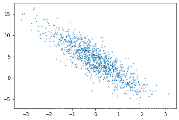
• 生成数据集：预先设置一个回归方程，通过对样本增加噪声来生成一个数据集，如图：
  

import torch
from IPython import display
from matplotlib import pyplot as plt
import numpy as np
import random

num_inputs = 2
num_examples = 1000

# w，b真实值
true_w = [2, -3.4]
true_b = 4.2

# 样本与标签
features = torch.randn(num_examples, num_inputs,
                      dtype=torch.float32)
labels = true_w[0] * features[:, 0] + true_w[1] * features[:, 1] + true_b
# 增加噪声
labels += torch.tensor(np.random.normal(0, 0.01, size=labels.size()),
                       dtype=torch.float32)

# 展示数据
plt.scatter(features[:, 1].numpy(), labels.numpy(), 1)                       

• 读取数据集
• 初始化参数 $\pmb{w},b$

# 将数据集按batchSize的数量进行随机划分
def data_iter(batch_size, features, labels):
    num_examples = len(features)
    indices = list(range(num_examples))
    random.shuffle(indices)  # 打乱原索引顺序
    for i in range(0, num_examples, batch_size):
        # 每次得到batchSize个数据（随机的）
        j = torch.LongTensor(indices[i: min(i + batch_size, num_examples)]) 
        yield  features.index_select(0, j), labels.index_select(0, j)  

batch_size = 10

# 生成权重ws(随机值)和截距b(0)的初始值
w = torch.tensor(np.random.normal(0, 0.01, (num_inputs, 1)), dtype=torch.float32)
b = torch.zeros(1, dtype=torch.float32)
# 需要更新梯度 
w.requires_grad_(requires_grad=True)
b.requires_grad_(requires_grad=True)

• 构建模型
• 损失函数与优化函数

# 线性模型
def linreg(X, w, b):
    return torch.mm(X, w) + b
    
# 损失函数：1/2(y_hat-y)^2
def squared_loss(y_hat, y): 
    return (y_hat - y.view(y_hat.size())) ** 2 / 2

# 优化函数:小批量随机梯度下降
def sgd(params, lr, batch_size): 
    for param in params:
        param.data -= lr * param.grad / batch_size

• 训练模型

lr = 0.03 # 梯度系数
num_epochs = 5 # 迭代次数

net = linreg
loss = squared_loss

for epoch in range(num_epochs):
    for X, y in data_iter(batch_size, features, labels):
        l = loss(net(X, w, b), y).sum() 
        l.backward()  # 得到梯度
        sgd([w, b], lr, batch_size)  # 优化
        w.grad.data.zero_() # 清空梯度记录
        b.grad.data.zero_()
    train_l = loss(net(features, w, b), labels)
    print('epoch %d, loss %f' % (epoch + 1, train_l.mean().item()))

>>> w, true_w, b, true_b
>(tensor([[ 1.9999],
         [-3.3993]], requires_grad=True),
 [2, -3.4],
 tensor([4.2000], requires_grad=True),
 4.2) # 结果近似相同，模型有效

 
 

3.pytorch实现线性回归

• 生成数据集过程同上
• 读取数据集

import torch
from torch import nn
import numpy as np
torch.manual_seed(1) # 设置随机数种子
# 设置默认数据类型为浮点数
torch.set_default_tensor_type('torch.FloatTensor')   
import torch.utils.data as Data

batch_size = 10
dataset = Data.TensorDataset(features, labels)
data_iter = Data.DataLoader(
      dataset = dataset,     # 形成 TensorDataset 的形式
      batch_size = batch_size, 
      shuffle = True,   # 随机采样数据
      num_workers = 2,  # 用多个进程导入数据
)

• 构造模型（以及三种方式构造序贯网络模型）

# 线性模型
class LinearNet(nn.Module):
    def __init__(self, n_feature):
        super(LinearNet, self).__init__()
        # torch.nn.Linear(in_features, out_features, bias=True)       
        self.linear = nn.Linear(n_feature, 1)  
    # 前向传播
    def forward(self, x):
        y = self.linear(x)
        return y

net = LinearNet(num_inputs) # 从零实现模型

# 下面是nn.Sequential函数使网络模型构造更为简化
# 方法一
net = nn.Sequential(
    nn.Linear(input_num,1)
    )
# 方法二
net = nn.Sequential()
net.add_module('linear',nn.Linear(input_num,1))
# 方法三
from collections import OrderedDict
net = nn.Sequential(OrderedDict([('linear',nn.Linear(input_num,1))]))

 
 

二、SoftMax回归和分类模型

1.SoftMax的概念

(1)基本表达式

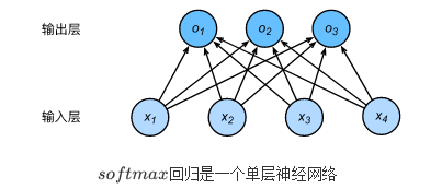
• softmax回归是一个单层神经网络，其输出值 $o_1,o_2,o_3$完全依赖于输入值 $x_1,x_2,x_3,x_4$，所以输出层是一个全连接层。

• 表达式为： $o_1=x_1w_{11}+x_2w_{21}+x_3w_{31}+x_4w_{41}+b_1\\ o_2=x_1w_{12}+x_2w_{22}+x_3w_{32}+x_4w_{42}+b_2\\ o_3=x_1w_{13}+x_2w_{23}+x_3w_{33}+x_4w_{43}+b_3$即： $o^{(i)}=x^{(i)}W+b$
  

• SoftMax回归通过 $o_1,o_2,o_3$的值进行分类。若 $o_1,o_2,o_3$分别为1，2，3，则选择值最大的标签作为预测类别，即预测为 $o_3$。

• 输出存在问题：

• 这些输出值与真实标签的离散值的误差难以衡量
  2.输出值的范围不确定，难以直观反映输出值的意义。

• 解决措施：SoftMax运算符，将输出值转换为正数且和为1( $\hat{y_1}+\hat{y_2}+\hat{y_3}=1$)的值： $\hat{y_1},\hat{y_2},\hat{y_3}=softmax(o_1,o_2,o_3)$ $\hat{y_1}=\frac{e^{o_1}}{\sum_{i=1}^3 e^{o_i}}， \hat{y_2}=\frac{e^{o_2}}{\sum_{i=1}^3 e^{o_i}}，\hat{y_1}=\frac{e^{o_3}}{\sum_{i=1}^3 e^{o_i}}$

  • softmax运算不改变预测的类别 $argmax o_i=argmax \hat{y_i}$

• 综上：softmax回归表达式为： $O=XW+b\\\hat{Y}=softmax(O)$
   

(2)损失函数

• 一般的平方损失函数（ $(\hat{y}^{(i)}-y^{(i)})^2/2$）对于分类正确而预测值不同的结果的损失计算不同，较为不符合模型正确分类的目的。因此改善方法是选择其他的损失计算方式：交叉熵。 $H(\hat{y}^{(i)},y^{(i)})=-\sum_{j=1}^qy^{(i)}_j log \hat{y}^{(i)}_j$其中 $y^{(i)}_j$是向量 $y^{(i)}$的元素（正确类别对应位置的元素为0，其余元素为1），因此 $H(\hat{y}^{(i)},y^{(i)})=-log \hat{y}^{(i)}_{y^(i)}$
• 通过以上过程，可以看出交叉熵只关信正确类别的预测率。
• 假设训练集样本数为 $n$，则交叉熵损失函数为： $l(\theta)=\frac{1}{n}\sum_{i=1}^nH(\hat{y}^{(i)},y^{(i)})$若每个样本仅存在一个物体/标签，则可以简化为： $l(\theta)=-\frac{1}{n}\sum^n_{i=1}log\hat{y}^{(i)}_{y^(i)}$
• 因为 $e^{-nl(\theta)}=\prod_{i=1}^n\hat{y}^{(i)}_{y^{(i)}}$，所以最小化交叉熵损失函数等价于最大化所有类别的联合预测概率。
   

(3)训练模型和预测

• 根据训练集得到softmax回归模型，输入样本可以预测输出类别的概率。一般情况下将预测概率最大的类别作为输出类别，与真实类别一致则说明预测正确。我们将通过准确率来评价模型的表现。
   
   

2.从零实现softmax模型

• 获得数据并初始化模型参数

import torch
import torchvision
import numpy as np
import sys
import d2l  # d2l是自用函数的一个包
sys.path.append("/home/hesci/input")
import os

batch_size = 256
# 训练集和测试集
train_iter, test_iter = d2l.load_data_fashion_mnist(batch_size, root='/home/kesci/input/FashionMNIST2065')

# 初始化模型参数
num_inputs = 784 # 输入层个数
num_outputs = 10 # 输出层个数

# weights初始值元素为服从正态分布的随机数
W = torch.tensor(np.random.normal(0, 0.01, (num_inputs, num_outputs)), dtype=torch.float)
# b初始值元素为0
b = torch.zeros(num_outputs, dtype=torch.float)

# 可以计算梯度
W.requires_grad_(requires_grad=True)
b.requires_grad_(requires_grad=True)

• softmax运算符： $\hat{y}_j=\frac{e^{o_j}}{\sum^3_{i=1}e^{o_i}}$
• softmax回归模型： $o^{(i)} =x^{(i)}W+b\\\hat{y}^{(i)} = softmax(o^{(i)})$

# softmax运算符
def softmax(X):
    X_exp = X.exp()
    partition = X_exp.sum(dim=1, keepdim=True) # dim为1，按照相同的行求和，并在结果中保留行特征
    return X_exp / partition

# 网络模型
def net(X):
    # torch.mm将两个矢量相乘
    return softmax(torch.mm(X.view((-1, num_inputs)), W) + b)

• 交叉熵损失函数： $l(\theta)=-\frac{1}{n}\sum^n_{i=1}log\hat{y}^{(i)}_{y^(i)}$
• 准确率

# 损失函数
# torch.gather(input,dim,index,out=None)或 y.gather(dim,index,out=None)
# 按照索引和维度的方向取出数据
def cross_entropy(y_hat, y):
    return - torch.log(y_hat.gather(1, y.view(-1, 1)))

# 准确率
def accuracy(y_hat, y):
    # y.argmax(dim)返回对应维度上最大值的索引
    return (y_hat.argmax(dim=1) == y).float().mean().item()

# 估计总体准确率
def evaluate_accuracy(data_iter, net):
    acc_sum, n = 0.0, 0
    for X, y in data_iter:
        acc_sum += (net(X).argmax(dim=1) == y).float().sum().item() 
        n += y.shape[0]
    return acc_sum / n

• 训练模型与预测

# 训练模型
num_epochs, lr = 5, 0.1

def train_ch3(net, train_iter, test_iter, loss, num_epochs, batch_size,params=None, lr=None, optimizer=None):
    for epoch in range(num_epochs):
        train_l_sum, train_acc_sum, n = 0.0, 0.0, 0
        for X, y in train_iter:
            y_hat = net(X)
            l = loss(y_hat, y).sum()
            
            # 梯度清零
            if optimizer is not None:
                optimizer.zero_grad()
            elif params is not None and params[0].grad is not None:
                for param in params:
                    param.grad.data.zero_()

            l.backward()
            if optimizer is None:
                d2l.sgd(params, lr, batch_size)
            else:
                optimizer.step() 
            train_l_sum += l.item()
            train_acc_sum += (y_hat.argmax(dim=1) == y).sum().item()
            n += y.shape[0]
        test_acc = evaluate_accuracy(test_iter, net)
        print('epoch %d, loss %.4f, train acc %.3f, test acc %.3f'
              % (epoch + 1, train_l_sum / n, train_acc_sum / n, test_acc))

train_ch3(net, train_iter, test_iter, cross_entropy, num_epochs, batch_size, [W, b], lr)

# 模型预测
X, y = iter(test_iter).next()
true_labels = d2l.get_fashion_mnist_labels(y.numpy())
pred_labels = d2l.get_fashion_mnist_labels(net(X).argmax(dim=1).numpy())
titles = [true + '\n' + pred for true, pred in zip(true_labels, pred_labels)]
d2l.show_fashion_mnist(X[0:9], titles[0:9]

 
 

3.pytorch实现softmax回归模型

• 导入数据与初始化参数

import torch
from torch import nn
from torch.nn import init
import numpy as np
import sys
sys.path.append("/home/kesci/input")

batch_size = 256
# 训练集与测试集
train_iter, test_iter = d2l.load_data_fashion_mnist(batch_size, root='/home/kesci/input/FashionMNIST2065')

# 初始化参数
init.normal_(net.linear.weight, mean=0, std=0.01) # weights
init.constant_(net.linear.bias, val=0) # b

• soft回归模型，构造网络

num_inputs = 784
num_outputs = 10

# 网络模型
# net = LinearNet(num_inputs, num_outputs)
class LinearNet(nn.Module):
    def __init__(self, num_inputs, num_outputs):
        super(LinearNet, self).__init__()
        self.linear = nn.Linear(num_inputs, num_outputs) 
    def forward(self, x): # x 的形状: (batch, 1, 28, 28)
        y = self.linear(x.view(x.shape[0], -1))
        return y
        
class FlattenLayer(nn.Module):
    def __init__(self):
        super(FlattenLayer, self).__init__()
    def forward(self, x): # x 的形状: (batch, *, *, ...)
        return x.view(x.shape[0], -1)

# 构建网络
from collections import OrderedDict
net = nn.Sequential(
        OrderedDict([
           ('flatten', FlattenLayer()),
           ('linear', nn.Linear(num_inputs, num_outputs))]) 
        )

• 损失函数与优化函数
• 训练模型

# 损失函数
# torch.nn.CrossEntropyLoss(weight=None, size_average=None, ignore_index=-100, reduce=None, reduction='mean')
loss = nn.CrossEntropyLoss()

# 优化函数
# torch.optim.SGD(params, lr=, momentum=0, dampening=0, weight_decay=0, nesterov=False)
optimizer = torch.optim.SGD(net.parameters(), lr=0.1)

# 训练模型
num_epochs = 5
d2l.train_ch3(net, train_iter, test_iter, loss, num_epochs, batch_size, None, None, optimizer)

 
 

三、多层感知机

1.多层感知机的概念

(1)基本构造

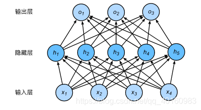
• 深度学习主要关注多层神经网络，多层感知机是多层神经网络的一种，是含有至少一个隐藏层的由全连接层组成的神经网络，且每个隐藏层的输出通过激活函数进行变换。
• 仅含一个隐藏层的多层感知机结构如下图所示。

• 表达公式—含单隐藏层的多层感知机： $\pmb{H}=\pmb{X}\pmb{W}_h+\pmb{b}_h\\ \pmb{O}=\pmb{H}\pmb{W}_o+\pmb{b}_o$
  • 给定样本 $\pmb{X}$，批量为 $n$。
  • 假设多层感知机只有一个隐藏层，隐藏单元有 $h$个，隐藏层变量(输出)为 $\pmb{H}$。
  • 隐藏层和输出层均为全连接层，所以设隐藏层权重参数和偏差参数为 $\pmb{W}_h,\pmb{b}_h$，输出层权重和偏差为 $\pmb{W}_o ,\pmb{b}_o$
• 可以将两个式子联立起来： $\pmb{O}=(\pmb{X}\pmb{W}_h+\pmb{b}_h)\pmb{W}_o+\pmb{b}_o=\pmb{X}\pmb{W}_h\pmb{W}_o+\pmb{b}_h\pmb{W}_o+\pmb{b}_o$
  • 由上式，虽然引入了隐藏层，但是经过变换后等价于一个单层神经网络。由此推导出，即使增加更多隐藏层，依然等价于仅含输出层的单层神经网络。
     

(2)激活函数

• 这种多层神经网络等价于单层神经网络的问题在于全连接层只是对数据进行仿射变换(线性变换+平移： $\vec{y}=w\vec{x}+b$)，多个仿射变换的叠加仍然是一个仿射变换（线性的叠加仍然是线性方程）。解决问题的一个方法是引入非线性变换。这个非线性函数被称为激活函数。
• 常用激活函数有：ReLU函数，Sigmoid函数和tanh函数。
  • 选择激活函数时，通用的激活函数是ReLU函数，计算量较小。在神经网络层数较多时尽量使用ReLU函数。但仅能在隐藏层使用。
  • sigmoid函数及其组合在分类器中效果更好。由于梯度消失问题，有时需要避免使用sigmodi函数和tanh函数。
     

ReLU函数

• $ReLU(x)=max(x,0)$
• 只保留正数元素，将负数元素归零
• .detach():返回相同数据的 tensor ,且 requires_grad=False
  • 这个新的tensor和原来的tensor是共用数据的，一者改变，另一者也会跟着改变，
  • 且新分离得到的tensor的require s_grad = False, 即不可求导的。
    避免原变量改变后求导结果改变，出现求导结果与数据对应不上的情况，
    如果要求导会直接报错

import torch
import numpy as np
import matplotlib.pyplot as plt
import sys
sys.path.append('/home/kesci/input')

# 绘图
def xyplot(x_vals,y_vals,name):
    #  .detach() 返回相同数据的 tensor ,且 requires_grad=False 
    """ 而且这个新的tensor和原来的tensor是共用数据的，一者改变，另一者也会跟着改变，
    而且新分离得到的tensor的require s_grad = False, 即不可求导的。
    避免原变量改变后求导结果改变，出现求导结果与数据对应不上的情况，
    如果要求导会直接报错"""
    plt.plot(x_vals.detach().numpy(),y_vals.detach().numpy())
    plt.xlabel('x')
    plt.ylabel(name + '(x)')

# 例子
# torch.arange(start,end,step):以start为首，以step为间隔，以end为结尾的数据（不含end)
x = torch.arange(-8.0, 8.0, 0.1, requires_grad=True)
y = x.relu()
xyplot(x,y,'relu')
>>> # (图如下所示)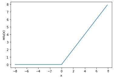

 

Sigmoid函数

• $sigmoid(x)=\frac{1}{1+e^{-x}}$：将元素的值变换到 $[0,1]$之间。
• sigmoid函数的导数： $sigmoid '(x)=sigmoid(x)(1-sigmoid(x))$

y = x.sigmoid()
xyplot(x,y,'sigmoid')
# 图如下所示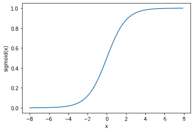

 

tanh函数

• $tanh(x)=\frac{1-e^{-2x}}{1+e^{-2x}}$：双曲正切函数。
  • 当输入值接近0时，tanh函数接近线性变换，关于原点对称。
• tanh函数的导函数： $tanh'(x)=1-tanh^2(x)$

# tanh函数
y = x.tanh()
xyplot(x, y, 'tanh')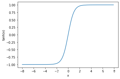

 

(3)表达式

• 多层感知机的层数和各隐藏层的隐藏单元个数都是超参数。
• 单隐藏层的多层感知机表达式： $\begin{aligned} \pmb{H}&=\phi(\pmb{X}\pmb{W}_h+\pmb{b}_h)\\ \pmb{O}&=\pmb{H}\pmb{W}_o+\pmb{b}_o \end{aligned}$ $\phi(x)$为激活函数
   

(4)从零实现多层感知机

• 初始化模型和参数

import torch
import numpy as np
import sys
import d2lzh1981 as d2l # 自定义的函数包
sys.path.append("/home/kesci/input")

# 获取数据集
batch_size = 256
train_iter, test_iter = d2l.load_data_fashion_mnist(batch_size,root='/home/kesci/input/FashionMNIST2065')

# 定义模型参数
num_inputs, num_outputs, num_hiddens = 784, 10, 256

# 初始化参数，w1，b1为隐藏层参数，w2，b2为输出层参数
W1 = torch.tensor(np.random.normal(0, 0.01, (num_inputs, num_hiddens)), dtype=torch.float)
b1 = torch.zeros(num_hiddens, dtype=torch.float)
W2 = torch.tensor(np.random.normal(0, 0.01, (num_hiddens, num_outputs)), dtype=torch.float)
b2 = torch.zeros(num_outputs, dtype=torch.float)

params = [W1, b1, W2, b2]
for param in params:
    param.requires_grad_(requires_grad=True)

• 激活函数，网络模型，损失函数

# 激活函数
def relu(X):
    return torch.max(input=X, other=torch.tensor(0.0))

# 网络模型
def net(X):
    X = X.view((-1, num_inputs))
    # torch.matmul()矩阵相乘
    H = relu(torch.matmul(X, W1) + b1) # 隐藏层输出
    return torch.matmul(H, W2) + b2 # 输出层

# 损失函数
# torch.nn.CrossEntropyLoss()：交叉熵损失函数
loss = torch.nn.CrossEntropyLoss()

# 训练
num_epochs, lr = 5, 100.0
d2l.train_ch3(net, train_iter, test_iter, loss, num_epochs, batch_size, params, lr)

# 输出
>>> epoch 1, loss 0.0030, train acc 0.718, test acc 0.810
epoch 2, loss 0.0019, train acc 0.823, test acc 0.802
epoch 3, loss 0.0017, train acc 0.845, test acc 0.806
epoch 4, loss 0.0015, train acc 0.856, test acc 0.804
epoch 5, loss 0.0014, train acc 0.865, test acc 0.844

(5)pytorch实现多层感知机

import torch
from torch import nn
from torch.nn import init
import numpy as np
import sys
sys.path.append("/home/kesci/input")
import d2lzh1981 as d2l # 自定义函数包

# 初始化参数
num_inputs, num_outputs, num_hiddens = 784, 10, 256
net = nn.Sequential(
        d2l.FlattenLayer(),
        nn.Linear(num_inputs, num_hiddens),  # 输入层输出
        nn.ReLU(),                           # 对上面的输出进行激活
        nn.Linear(num_hiddens, num_outputs), # 隐藏层输出
        )    
for params in net.parameters():
    init.normal_(params, mean=0, std=0.01)

# 训练
batch_size = 256
# 训练集
train_iter, test_iter = d2l.load_data_fashion_mnist(batch_size,root='/home/kesci/input/FashionMNIST2065')
# 损失函数：交叉熵
loss = torch.nn.CrossEntropyLoss()
# 优化函数
optimizer = torch.optim.SGD(net.parameters(), lr=0.5)

num_epochs = 5
d2l.train_ch3(net, train_iter, test_iter, loss, num_epochs, batch_size, None, None, optimizer)

# 输出
>>> epoch 1, loss 0.0031, train acc 0.707, test acc 0.776
epoch 2, loss 0.0019, train acc 0.820, test acc 0.771
epoch 3, loss 0.0016, train acc 0.845, test acc 0.833
epoch 4, loss 0.0015, train acc 0.854, test acc 0.843
epoch 5, loss 0.0014, train acc 0.865, test acc 0.848