动手学 Task06批量归一化和残差网络+凸优化+梯度下降

批量归一化和残差网络

批量归一化（BatchNormalization）
对输入的标准化（浅层模型）
处理后的任意一个特征在数据集中所有样本上的均值为0、标准差为1。
标准化处理输入数据使各个特征的分布相近

批量归一化（深度模型）
利用小批量上的均值和标准差，不断调整神经网络中间输出，从而使整个神经网络在各层的中间输出的数值更稳定。

1.对全连接层做批量归一化
位置：全连接层中的仿射变换和激活函数之间。

2.对卷积层做批量归⼀化
位置：卷积计算之后、应⽤激活函数之前。
如果卷积计算输出多个通道，我们需要对这些通道的输出分别做批量归一化，且每个通道都拥有独立的拉伸和偏移参数。
计算：对单通道，batchsize=m,卷积计算输出=pxq 对该通道中m×p×q个元素同时做批量归一化,使用相同的均值和方差。
3.预测时的批量归⼀化
训练：以batch为单位,对每个batch计算均值和方差。
预测：用移动平均估算整个训练数据集的样本均值和方差。
代码实现：

import time
import torch
from torch import nn, optim
import torch.nn.functional as F
import torchvision
import sys
sys.path.append("/home/kesci/input/") 
import d2lzh1981 as d2l
device = torch.device('cuda' if torch.cuda.is_available() else 'cpu')

def batch_norm(is_training, X, gamma, beta, moving_mean, moving_var, eps, momentum):
    # 判断当前模式是训练模式还是预测模式
    if not is_training:
        # 如果是在预测模式下，直接使用传入的移动平均所得的均值和方差
        X_hat = (X - moving_mean) / torch.sqrt(moving_var + eps)
    else:
        assert len(X.shape) in (2, 4)
        if len(X.shape) == 2:
            # 使用全连接层的情况，计算特征维上的均值和方差
            mean = X.mean(dim=0)
            var = ((X - mean) ** 2).mean(dim=0)
        else:
            # 使用二维卷积层的情况，计算通道维上（axis=1）的均值和方差。这里我们需要保持
            # X的形状以便后面可以做广播运算
            mean = X.mean(dim=0, keepdim=True).mean(dim=2, keepdim=True).mean(dim=3, keepdim=True)
            var = ((X - mean) ** 2).mean(dim=0, keepdim=True).mean(dim=2, keepdim=True).mean(dim=3, keepdim=True)
        # 训练模式下用当前的均值和方差做标准化
        X_hat = (X - mean) / torch.sqrt(var + eps)
        # 更新移动平均的均值和方差
        moving_mean = momentum * moving_mean + (1.0 - momentum) * mean
        moving_var = momentum * moving_var + (1.0 - momentum) * var
    Y = gamma * X_hat + beta  # 拉伸和偏移
    return Y, moving_mean, moving_var

class BatchNorm(nn.Module):
    def __init__(self, num_features, num_dims):
        super(BatchNorm, self).__init__()
        if num_dims == 2:
            shape = (1, num_features) #全连接层输出神经元
        else:
            shape = (1, num_features, 1, 1)  #通道数
        # 参与求梯度和迭代的拉伸和偏移参数，分别初始化成0和1
        self.gamma = nn.Parameter(torch.ones(shape))
        self.beta = nn.Parameter(torch.zeros(shape))
        # 不参与求梯度和迭代的变量，全在内存上初始化成0
        self.moving_mean = torch.zeros(shape)
        self.moving_var = torch.zeros(shape)

    def forward(self, X):
        # 如果X不在内存上，将moving_mean和moving_var复制到X所在显存上
        if self.moving_mean.device != X.device:
            self.moving_mean = self.moving_mean.to(X.device)
            self.moving_var = self.moving_var.to(X.device)
        # 保存更新过的moving_mean和moving_var, Module实例的traning属性默认为true, 调用.eval()后设成false
        Y, self.moving_mean, self.moving_var = batch_norm(self.training, 
            X, self.gamma, self.beta, self.moving_mean,
            self.moving_var, eps=1e-5, momentum=0.9)
        return Y

基于LeNet的应用

net = nn.Sequential(
            nn.Conv2d(1, 6, 5), # in_channels, out_channels, kernel_size
            BatchNorm(6, num_dims=4),
            nn.Sigmoid(),
            nn.MaxPool2d(2, 2), # kernel_size, stride
            nn.Conv2d(6, 16, 5),
            BatchNorm(16, num_dims=4),
            nn.Sigmoid(),
            nn.MaxPool2d(2, 2),
            d2l.FlattenLayer(),
            nn.Linear(16*4*4, 120),
            BatchNorm(120, num_dims=2),
            nn.Sigmoid(),
            nn.Linear(120, 84),
            BatchNorm(84, num_dims=2),
            nn.Sigmoid(),
            nn.Linear(84, 10)
        )
print(net)

#batch_size = 256  
##cpu要调小batchsize
batch_size=16

def load_data_fashion_mnist(batch_size, resize=None, root='/home/kesci/input/FashionMNIST2065'):
    """Download the fashion mnist dataset and then load into memory."""
    trans = []
    if resize:
        trans.append(torchvision.transforms.Resize(size=resize))
    trans.append(torchvision.transforms.ToTensor())
    
    transform = torchvision.transforms.Compose(trans)
    mnist_train = torchvision.datasets.FashionMNIST(root=root, train=True, download=True, transform=transform)
    mnist_test = torchvision.datasets.FashionMNIST(root=root, train=False, download=True, transform=transform)

    train_iter = torch.utils.data.DataLoader(mnist_train, batch_size=batch_size, shuffle=True, num_workers=2)
    test_iter = torch.utils.data.DataLoader(mnist_test, batch_size=batch_size, shuffle=False, num_workers=2)

    return train_iter, test_iter
train_iter, test_iter = load_data_fashion_mnist(batch_size)

lr, num_epochs = 0.001, 5
optimizer = torch.optim.Adam(net.parameters(), lr=lr)
d2l.train_ch5(net, train_iter, test_iter, batch_size, optimizer, device, num_epochs)

简洁实现：

net = nn.Sequential(
            nn.Conv2d(1, 6, 5), # in_channels, out_channels, kernel_size
            nn.BatchNorm2d(6),
            nn.Sigmoid(),
            nn.MaxPool2d(2, 2), # kernel_size, stride
            nn.Conv2d(6, 16, 5),
            nn.BatchNorm2d(16),
            nn.Sigmoid(),
            nn.MaxPool2d(2, 2),
            d2l.FlattenLayer(),
            nn.Linear(16*4*4, 120),
            nn.BatchNorm1d(120),
            nn.Sigmoid(),
            nn.Linear(120, 84),
            nn.BatchNorm1d(84),
            nn.Sigmoid(),
            nn.Linear(84, 10)
        )

optimizer = torch.optim.Adam(net.parameters(), lr=lr)
d2l.train_ch5(net, train_iter, test_iter, batch_size, optimizer, device, num_epochs)

残差网络（ResNet）
深度学习的问题：深度CNN网络达到一定深度后再一味地增加层数并不能带来进一步地分类性能提高，反而会招致网络收敛变得更慢，准确率也变得更差。

残差块（Residual Block）
恒等映射：
左边：f(x)=x
右边：f(x)-x=0 （易于捕捉恒等映射的细微波动）

实现：

class Residual(nn.Module):  # 本类已保存在d2lzh_pytorch包中方便以后使用
    #可以设定输出通道数、是否使用额外的1x1卷积层来修改通道数以及卷积层的步幅。
    def __init__(self, in_channels, out_channels, use_1x1conv=False, stride=1):
        super(Residual, self).__init__()
        self.conv1 = nn.Conv2d(in_channels, out_channels, kernel_size=3, padding=1, stride=stride)
        self.conv2 = nn.Conv2d(out_channels, out_channels, kernel_size=3, padding=1)
        if use_1x1conv:
            self.conv3 = nn.Conv2d(in_channels, out_channels, kernel_size=1, stride=stride)
        else:
            self.conv3 = None
        self.bn1 = nn.BatchNorm2d(out_channels)
        self.bn2 = nn.BatchNorm2d(out_channels)

    def forward(self, X):
        Y = F.relu(self.bn1(self.conv1(X)))
        Y = self.bn2(self.conv2(Y))
        if self.conv3:
            X = self.conv3(X)
        return F.relu(Y + X)

blk = Residual(3, 3)
X = torch.rand((4, 3, 6, 6))
blk(X).shape # torch.Size([4, 3, 6, 6])

blk = Residual(3, 6, use_1x1conv=True, stride=2)
blk(X).shape # torch.Size([4, 6, 3, 3])

ResNet模型
卷积(64,7x7,3)
批量一体化
最大池化(3x3,2)

残差块x4 (通过步幅为2的残差块在每个模块之间减小高和宽)

全局平均池化

全连接
实现：

net = nn.Sequential(
        nn.Conv2d(1, 64, kernel_size=7, stride=2, padding=3),
        nn.BatchNorm2d(64), 
        nn.ReLU(),
        nn.MaxPool2d(kernel_size=3, stride=2, padding=1))

def resnet_block(in_channels, out_channels, num_residuals, first_block=False):
    if first_block:
        assert in_channels == out_channels # 第一个模块的通道数同输入通道数一致
    blk = []
    for i in range(num_residuals):
        if i == 0 and not first_block:
            blk.append(Residual(in_channels, out_channels, use_1x1conv=True, stride=2))
        else:
            blk.append(Residual(out_channels, out_channels))
    return nn.Sequential(*blk)

net.add_module("resnet_block1", resnet_block(64, 64, 2, first_block=True))
net.add_module("resnet_block2", resnet_block(64, 128, 2))
net.add_module("resnet_block3", resnet_block(128, 256, 2))
net.add_module("resnet_block4", resnet_block(256, 512, 2))

net.add_module("global_avg_pool", d2l.GlobalAvgPool2d()) # GlobalAvgPool2d的输出: (Batch, 512, 1, 1)
net.add_module("fc", nn.Sequential(d2l.FlattenLayer(), nn.Linear(512, 10))) 

X = torch.rand((1, 1, 224, 224))
for name, layer in net.named_children():
    X = layer(X)
    print(name, ' output shape:\t', X.shape)

lr, num_epochs = 0.001, 5
optimizer = torch.optim.Adam(net.parameters(), lr=lr)
d2l.train_ch5(net, train_iter, test_iter, batch_size, optimizer, device, num_epochs)

稠密连接网络（DenseNet）
主要构建模块：
稠密块（dense block）： 定义了输入和输出是如何连结的。
过渡层（transition layer）：用来控制通道数，使之不过大。

实现：

def conv_block(in_channels, out_channels):
    blk = nn.Sequential(nn.BatchNorm2d(in_channels), 
                        nn.ReLU(),
                        nn.Conv2d(in_channels, out_channels, kernel_size=3, padding=1))
    return blk

class DenseBlock(nn.Module):
    def __init__(self, num_convs, in_channels, out_channels):
        super(DenseBlock, self).__init__()
        net = []
        for i in range(num_convs):
            in_c = in_channels + i * out_channels
            net.append(conv_block(in_c, out_channels))
        self.net = nn.ModuleList(net)
        self.out_channels = in_channels + num_convs * out_channels # 计算输出通道数

    def forward(self, X):
        for blk in self.net:
            Y = blk(X)
            X = torch.cat((X, Y), dim=1)  # 在通道维上将输入和输出连结
        return X

blk = DenseBlock(2, 3, 10)
X = torch.rand(4, 3, 8, 8)
Y = blk(X)
Y.shape # torch.Size([4, 23, 8, 8])

def transition_block(in_channels, out_channels):
    blk = nn.Sequential(
            nn.BatchNorm2d(in_channels), 
            nn.ReLU(),
            nn.Conv2d(in_channels, out_channels, kernel_size=1),
            nn.AvgPool2d(kernel_size=2, stride=2))
    return blk

blk = transition_block(23, 10)
blk(Y).shape # torch.Size([4, 10, 4, 4])

凸优化

优化与深度学习
优化与估计
尽管优化方法可以最小化深度学习中的损失函数值，但本质上优化方法达到的目标与深度学习的目标并不相同。

优化方法目标：训练集损失函数值
深度学习目标：测试集损失函数值（泛化性）

优化在深度学习中的挑战

1. 局部最小值
2. 鞍点
3. 梯度消失
   

def f(x):
    return x * np.cos(np.pi * x)

d2l.set_figsize((4.5, 2.5))
x = np.arange(-1.0, 2.0, 0.1)
fig,  = d2l.plt.plot(x, f(x))
fig.axes.annotate('local minimum', xy=(-0.3, -0.25), xytext=(-0.77, -1.0),
                  arrowprops=dict(arrowstyle='->'))
fig.axes.annotate('global minimum', xy=(1.1, -0.95), xytext=(0.6, 0.8),
                  arrowprops=dict(arrowstyle='->'))
d2l.plt.xlabel('x')
d2l.plt.ylabel('f(x)');

鞍点

x = np.arange(-2.0, 2.0, 0.1)
fig, = d2l.plt.plot(x, x**3)
fig.axes.annotate('saddle point', xy=(0, -0.2), xytext=(-0.52, -5.0),
                  arrowprops=dict(arrowstyle='->'))
d2l.plt.xlabel('x')
d2l.plt.ylabel('f(x)');

x, y = np.mgrid[-1: 1: 31j, -1: 1: 31j]
z = x**2 - y**2

d2l.set_figsize((6, 4))
ax = d2l.plt.figure().add_subplot(111, projection='3d')
ax.plot_wireframe(x, y, z, **{'rstride': 2, 'cstride': 2})
ax.plot([0], [0], [0], 'ro', markersize=10)
ticks = [-1,  0, 1]
d2l.plt.xticks(ticks)
d2l.plt.yticks(ticks)
ax.set_zticks(ticks)
d2l.plt.xlabel('x')
d2l.plt.ylabel('y');

梯度消失

x = np.arange(-2.0, 5.0, 0.01)
fig, = d2l.plt.plot(x, np.tanh(x))
d2l.plt.xlabel('x')
d2l.plt.ylabel('f(x)')
fig.axes.annotate('vanishing gradient', (4, 1), (2, 0.0) ,arrowprops=dict(arrowstyle='->'))

性质

1. 无局部极小值
2. 与凸集的关系
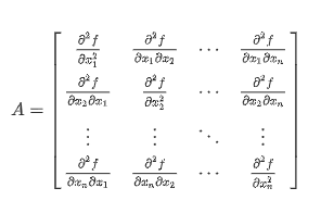
3. 二阶条件
   
   

梯度下降

一维梯度下降
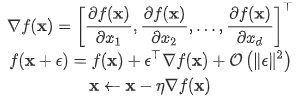
证明：沿梯度反方向移动自变量可以减小函数值

多维梯度下降

def train_2d(trainer, steps=20):
    x1, x2 = -5, -2
    results = [(x1, x2)]
    for i in range(steps):
        x1, x2 = trainer(x1, x2)
        results.append((x1, x2))
    print('epoch %d, x1 %f, x2 %f' % (i + 1, x1, x2))
    return results

def show_trace_2d(f, results): 
    d2l.plt.plot(*zip(*results), '-o', color='#ff7f0e')
    x1, x2 = np.meshgrid(np.arange(-5.5, 1.0, 0.1), np.arange(-3.0, 1.0, 0.1))
    d2l.plt.contour(x1, x2, f(x1, x2), colors='#1f77b4')
    d2l.plt.xlabel('x1')
    d2l.plt.ylabel('x2')

eta = 0.1

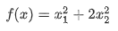
def f_2d(x1, x2):  # 目标函数
    return x1 ** 2 + 2 * x2 ** 2

def gd_2d(x1, x2):
    return (x1 - eta * 2 * x1, x2 - eta * 4 * x2)

show_trace_2d(f_2d, train_2d(gd_2d))

自适应方法

c = 0.5

def f(x):
    return np.cosh(c * x)  # Objective

def gradf(x):
    return c * np.sinh(c * x)  # Derivative

def hessf(x):
    return c**2 * np.cosh(c * x)  # Hessian

# Hide learning rate for now
def newton(eta=1):
    x = 10
    results = [x]
    for i in range(10):
        x -= eta * gradf(x) / hessf(x)
        results.append(x)
    print('epoch 10, x:', x)
    return results

show_trace(newton())

随机梯度下降
随机梯度下降参数更新

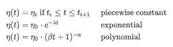
动态学习率