sklearn中线性回归API介绍、波士顿房价预测

一、线性回归api

（1）通过正规方程优化

sklearn.linear_model.LinearRegression(fit_intercept=True)

• 通过正规方程优化
• 参数
  • fit_intercept：是否计算偏置
• 属性
  • LinearRegression.coef_：回归系数
  • LinearRegression.intercept_：偏置

（2）通过梯度下降方法优化

sklearn.linear_model.SGDRegressor(loss="squared_loss", fit_intercept=True, learning_rate ='invscaling', eta0=0.01)

• SGDRegressor类实现了随机梯度下降学习，它支持不同的loss函数和正则化惩罚项来拟合线性回归模型。
• 参数：
  • loss:损失类型
    • loss=”squared_loss”: 普通最小二乘法
  • fit_intercept：是否计算偏置
  • learning_rate : string, optional
    • 学习率填充
    • 'constant': eta = eta0
    • 'optimal': eta = 1.0 / (alpha * (t + t0))  默认
    • 'invscaling': eta = eta0 / pow(t, power_t)
      • power_t=0.25:存在父类当中
    • 对于一个常数值的学习率来说，可以使用learning_rate=’constant’ ，并使用eta0来指定学习率。
• 属性：
  • SGDRegressor.coef_：回归系数
  • SGDRegressor.intercept_：偏置

二、波士顿房价预测案例

（1）数据内容

（2）分析

回归当中的数据大小不一致，是否会导致结果影响较大。所以需要做标准化处理。

整个过程可以概括为以下三个部分：

• 数据分割与标准化处理
• 回归预测
• 线性回归的算法效果评估

（3） 回归性能评估

均方误差(Mean Squared Error)MSE)评价机制：

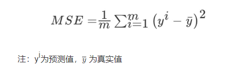
API：sklearn.metrics.mean_squared_error(y_true, y_pred)

• 均方误差回归损失
• y_true:真实值
• y_pred:预测值
• return:浮点数结果

"""
# 数据获取
# 数据基本处理
# 分割数据
# 特征工程
# 机器学习-线性回归
# 模型评估
"""
from sklearn.datasets import load_boston
from sklearn.model_selection import train_test_split
from sklearn.preprocessing import StandardScaler
from sklearn.linear_model import LinearRegression,SGDRegressor
from sklearn.metrics import mean_squared_error


def liner_model_1():
    """
    线性回归：正规方程
    """
    # 数据获取
    boston = load_boston()
    
    # 分割数据
    x_train, x_test, y_train,y_test = train_test_split(boston.data, boston.target, test_size=0.2) 
    
    # 特征工程
    transfer = StandardScaler()
    x_train = transfer.fit_transform(x_train)
    x_test = transfer.transform(x_test)
    
    # 机器学习-线性回归
    estimator = LinearRegression()
    estimator.fit(x_train, y_train)
    
    print("模型的偏置是：", estimator.intercept_)
    print("模型的系数是：", estimator.coef_)
    # 模型评估
    y_pred = estimator.predict(x_test)
    print('预测值是：',y_pred)
    
    # 均方误差
    mse = mean_squared_error(y_test, y_pred)
    print('均方误差为：',mse)
    
    
def liner_model_2():
    """
    线性回归：梯度下降
    """
    # 数据获取
    boston = load_boston()
    
    # 分割数据
    x_train, x_test, y_train,y_test = train_test_split(boston.data, boston.target, test_size=0.2) 
    
    # 特征工程
    transfer = StandardScaler()
    x_train = transfer.fit_transform(x_train)
    x_test = transfer.transform(x_test)
    
    # 机器学习-线性回归
    estimator = SGDRegressor(max_iter=2000,learning_rate="constant",eta0=0.0001)
    estimator.fit(x_train, y_train)
    
    print("模型的偏置是：", estimator.intercept_)
    print("模型的系数是：", estimator.coef_)
    # 模型评估
    y_pred = estimator.predict(x_test)
    print('预测值是：',y_pred)
    
    # 均方误差
    mse = mean_squared_error(y_test, y_pred)
    print('均方误差为：',mse)
    
liner_model_1()
print("*************************************************************")
liner_model_2()