深度学习_经典网络_AlexNet

一.AlexNet模型介绍

AlexNet是由 $Alex$ $Krizhevsky$提出的首个应用于图像分类的深层卷积神经网络，该网络在2012年ILSVRC（ImageNet Large Scale Visual Recognition Competition）图像分类竞赛中以15.3%的top-5测试错误率赢得第一名。 AlexNet使用GPU代替CPU进行运算，使得在可接受的时间范围内模型结构能够更加复杂，它的出现证明了深层卷积神经网络在复杂模型下的有效性，使CNN在计算机视觉中流行开来，直接或间接地引发了深度学习的热潮。

二.模型结构

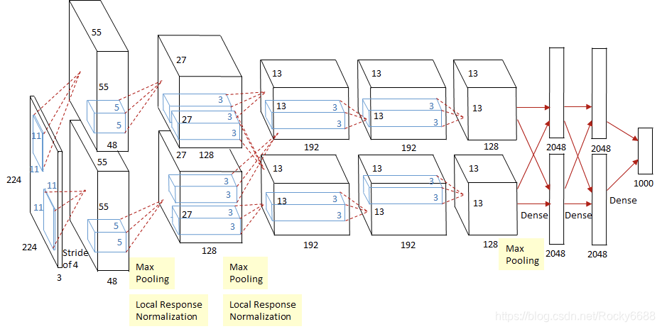
如上图所示，除去下采样（池化层）和局部响应规范化操作（Local Responsible Normalization，LRN），AlexNet一共包含8层，前5层由卷积层组成，而剩下的3层为全连接层。网络结构分为上下两层，分别对应两个GPU的操作过程，除了中间某些层（C₃卷积层和F_6-8全连接层会有GPU间的交互），其他层两个GPU分别计算结果。最后一层全连接层的输出作为softmax的输入，得到1000个图像分类标签对应的概率值。除去GPU并行结构的设计，AlexNet网络结构和LeNet十分相似。

三.AlexNet网络参数配置

网络层	输入尺寸	核尺寸	输出尺寸	可训练参数量
卷积层 $C_1$ $^*$	$224\times224\times3$	$11\times11\times96/4$	$55\times55\times96$	$(11\times11\times3+1)\times48\times2$
下采样层 $S_{max}$ $^*$	$55\times55\times96$	$3\times3/2$	$27\times27\times96$	0
卷积层 $C_2$	$27\times27\times96$	$5\times5\times256/1$	$27\times27\times256$	$(5\times5\times48+1)\times128\times2$
下采样层 $S_{max}$	$27\times27\times256$	$3\times3/2$	$13\times13\times256$	0
卷积层 $C_3$ $^*$	$13\times13\times256$	$3\times3\times384$	$13\times13\times384$	$(3\times3\times256+1)\times192\times2$
卷积层 $C_4$	$13\times13\times384$	$3\times3\times384$	$13\times13\times384$	$(3\times3\times192+1)\times192\times2$
卷积层 $C_5$	$13\times13\times384$	$3\times3\times256/1$	$13\times13\times256$	$(3\times3\times192+1)\times128\times2$
下采样层 $S_{max}$	$13\times13\times256$	$3\times3/2$	$6\times6\times256$	0
全连接层 $F_6$ $^*$	$6\times6\times256$	$9216\times4096$	$1\times1\times4096$	$(9216+1)\times2048\times2$
全连接层 $F_7$	$1\times1\times4096$	$4096\times4096$	$1\times1\times4096$	$(4096+1)\times2048\times2$
全连接层 $F_8$	$1\times1\times4096$	$4096\times1000$	$1\times1\times1000$	$(4096+1)\times1000\times2$

下面是相应的参数的代码：

def create(self):
        """Create the network graph."""
        # 1st Layer: Conv (w ReLu) -> Lrn -> Pool
        conv1 = conv(self.X, 11, 11, 96, 4, 4, padding='VALID', name='conv1')
        norm1 = lrn(conv1, 2, 2e-05, 0.75, name='norm1')
        pool1 = max_pool(norm1, 3, 3, 2, 2, padding='VALID', name='pool1')
        
        # 2nd Layer: Conv (w ReLu)  -> Lrn -> Pool with 2 groups
        conv2 = conv(pool1, 5, 5, 256, 1, 1, groups=2, name='conv2')
        norm2 = lrn(conv2, 2, 2e-05, 0.75, name='norm2')
        pool2 = max_pool(norm2, 3, 3, 2, 2, padding='VALID', name='pool2')
        
        # 3rd Layer: Conv (w ReLu)
        conv3 = conv(pool2, 3, 3, 384, 1, 1, name='conv3')

        # 4th Layer: Conv (w ReLu) splitted into two groups
        conv4 = conv(conv3, 3, 3, 384, 1, 1, groups=2, name='conv4')

        # 5th Layer: Conv (w ReLu) -> Pool splitted into two groups
        conv5 = conv(conv4, 3, 3, 256, 1, 1, groups=2, name='conv5')
        pool5 = max_pool(conv5, 3, 3, 2, 2, padding='VALID', name='pool5')

        # 6th Layer: Flatten -> FC (w ReLu) -> Dropout
        flattened = tf.reshape(pool5, [-1, 6*6*256])
        fc6 = fc(flattened, 6*6*256, 4096, name='fc6')
        dropout6 = dropout(fc6, self.KEEP_PROB)

        # 7th Layer: FC (w ReLu) -> Dropout
        fc7 = fc(dropout6, 4096, 4096, name='fc7')
        dropout7 = dropout(fc7, self.KEEP_PROB)

        # 8th Layer: FC and return unscaled activations
        self.fc8 = fc(dropout7, 4096, self.NUM_CLASSES, relu=False, name='fc8')

四.模型特点

1. 所有卷积层都使用ReLU作为非线性映射函数，使模型收敛速度更快。
2. 在多个GPU上进行模型的训练，不但可以提高模型的训练速度，还能提升数据的使用规模。
3. 使用LRN对局部的特征进行归一化，结果作为ReLU激活函数的输入能有效降低错误率。
4. 重叠最大池化（overlapping max pooling），即池化范围z与步长s存在关系 $z > s$(如S_max中核尺寸为 $3 \times 3 /2$)，避免平均池化（average pooling）的平均效应。
5. 使用随机丢弃技术（dropout）选择型地忽略训练中的单个神经元，避免模型的过拟合。