程序所用文件:https://files.cnblogs.com/files/henuliulei/%E5%9B%9E%E5%BD%92%E5%88%86%E7%B1%BB%E6%95%B0%E6%8D%AE.zip
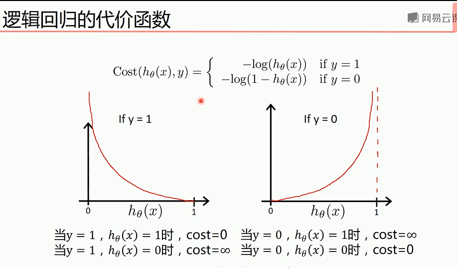
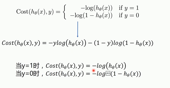
概念
代价函数关于参数的偏导
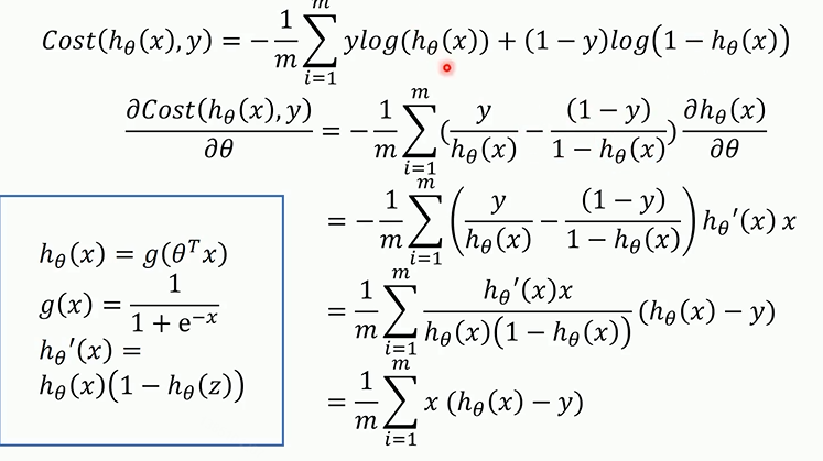
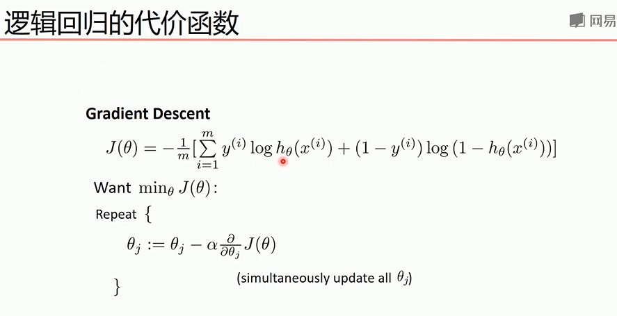
梯度下降法最终的推导公式如下

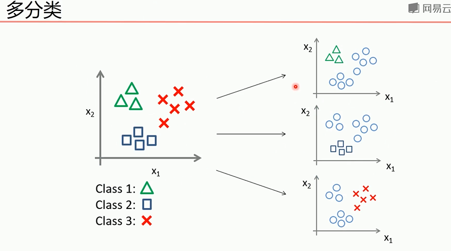
多分类问题可以转为2分类问题
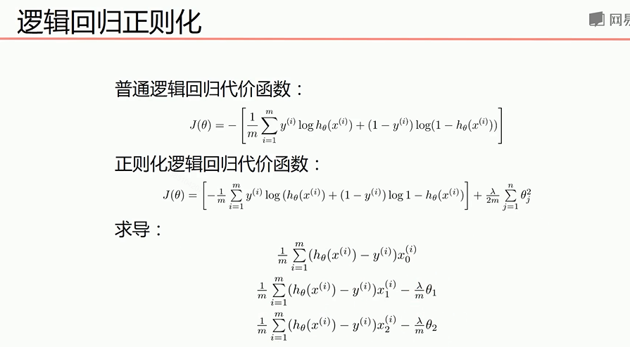
正则化处理可以防止过拟合,下面是正则化后的代价函数和求导后的式子
正确率和召回率F1指标


我们希望自己预测的结果希望更准确那么查准率就更高,如果希望更获得更多数量的正确结果,那么查全率更重要,综合考虑可以用F1指标
梯度下降法实现线性逻辑回归
  1 import matplotlib.pyplot as plt
  2 import numpy as np
  3 from sklearn.metrics import classification_report#分类
  4 from sklearn import preprocessing#预测
  5 # 数据是否需要标准化
  6 scale = True#True是需要,False是不需要,标准化后效果更好,标准化之前可以画图看出可视化结果
  7 scale = False
  8 # 载入数据
  9 data = np.genfromtxt("LR-testSet.csv", delimiter=",")
 10 x_data = data[:, :-1]
 11 y_data = data[:, -1]
 12
 13 def plot():
 14     x0 = []
 15     x1 = []
 16     y0 = []
 17     y1 = []
 18     # 切分不同类别的数据
 19     for i in range(len(x_data)):
 20         if y_data[i] == 0:
 21             x0.append(x_data[i, 0])
 22             y0.append(x_data[i, 1])
 23         else:
 24             x1.append(x_data[i, 0])
 25             y1.append(x_data[i, 1])
 26
 27     # 画图
 28     scatter0 = plt.scatter(x0, y0, c='b', marker='o')
 29     scatter1 = plt.scatter(x1, y1, c='r', marker='x')
 30     # 画图例
 31     plt.legend(handles=[scatter0, scatter1], labels=['label0', 'label1'], loc='best')
 32
 33
 34 plot()
 35 plt.show()
 36 # 数据处理,添加偏置项
 37 x_data = data[:,:-1]
 38 y_data = data[:,-1,np.newaxis]
 39
 40 print(np.mat(x_data).shape)
 41 print(np.mat(y_data).shape)
 42 # 给样本添加偏置项
 43 X_data = np.concatenate((np.ones((100,1)),x_data),axis=1)
 44 print(X_data.shape)
 45
 46 def sigmoid(x):
 47     return 1.0 / (1 + np.exp(-x))
 48
 49 def cost(xMat, yMat, ws):
 50     left = np.multiply(yMat, np.log(sigmoid(xMat * ws)))
 51     right = np.multiply(1 - yMat, np.log(1 - sigmoid(xMat * ws)))
 52     return np.sum(left + right) / -(len(xMat))
 53
 54 def gradAscent(xArr, yArr):
 55     if scale == True:
 56         xArr = preprocessing.scale(xArr)
 57     xMat = np.mat(xArr)
 58     yMat = np.mat(yArr)
 59
 60     lr = 0.001
 61     epochs = 10000
 62     costList = []
 63     # 计算数据行列数
 64     # 行代表数据个数,列代表权值个数
 65     m, n = np.shape(xMat)
 66     # 初始化权值
 67     ws = np.mat(np.ones((n, 1)))
 68
 69     for i in range(epochs + 1):
 70         # xMat和weights矩阵相乘
 71         h = sigmoid(xMat * ws)
 72         # 计算误差
 73         ws_grad = xMat.T * (h - yMat) / m
 74         ws = ws - lr * ws_grad
 75
 76         if i % 50 == 0:
 77             costList.append(cost(xMat, yMat, ws))
 78     return ws, costList
 79 # 训练模型,得到权值和cost值的变化
 80 ws,costList = gradAscent(X_data, y_data)
 81 print(ws)
 82 if scale == False:
 83     # 画图决策边界
 84     plot()
 85     x_test = [[-4],[3]]
 86     y_test = (-ws[0] - x_test*ws[1])/ws[2]
 87     plt.plot(x_test, y_test, 'k')
 88     plt.show()
 89 # 画图 loss值的变化
 90 x = np.linspace(0, 10000, 201)
 91 plt.plot(x, costList, c='r')
 92 plt.title('Train')
 93 plt.xlabel('Epochs')
 94 plt.ylabel('Cost')
 95 plt.show()
 96 # 预测
 97 def predict(x_data, ws):
 98     if scale == True:
 99         x_data = preprocessing.scale(x_data)
100     xMat = np.mat(x_data)
101     ws = np.mat(ws)
102     return [1 if x >= 0.5 else 0 for x in sigmoid(xMat*ws)]
103
104 predictions = predict(X_data, ws)
105
106 print(classification_report(y_data, predictions))#计算预测的分
sklearn实现线性逻辑回归
 1 import matplotlib.pyplot as plt
 2 import numpy as np
 3 from sklearn.metrics import classification_report
 4 from sklearn import preprocessing
 5 from sklearn import linear_model
 6 # 数据是否需要标准化
 7 scale = False
 8 # 载入数据
 9 data = np.genfromtxt("LR-testSet.csv", delimiter=",")
10 x_data = data[:, :-1]
11 y_data = data[:, -1]
12
13 def plot():
14     x0 = []
15     x1 = []
16     y0 = []
17     y1 = []
18     # 切分不同类别的数据
19     for i in range(len(x_data)):
20         if y_data[i] == 0:
21             x0.append(x_data[i, 0])
22             y0.append(x_data[i, 1])
23         else:
24             x1.append(x_data[i, 0])
25             y1.append(x_data[i, 1])
26
27     # 画图
28     scatter0 = plt.scatter(x0, y0, c='b', marker='o')
29     scatter1 = plt.scatter(x1, y1, c='r', marker='x')
30     # 画图例
31     plt.legend(handles=[scatter0, scatter1], labels=['label0', 'label1'], loc='best')
32
33 plot()
34 plt.show()
35 logistic = linear_model.LogisticRegression()
36 logistic.fit(x_data, y_data)
37 if scale == False:
38     # 画图决策边界
39     plot()
40     x_test = np.array([[-4],[3]])
41     y_test = (-logistic.intercept_ - x_test*logistic.coef_[0][0])/logistic.coef_[0][1]
42     plt.plot(x_test, y_test, 'k')
43     plt.show()
44 predictions = logistic.predict(x_data)
45
46 print(classification_report(y_data, predictions))
梯度下降法实现非线性逻辑回归
  1 import matplotlib.pyplot as plt
  2 import numpy as np
  3 from sklearn.metrics import classification_report
  4 from sklearn import preprocessing
  5 from sklearn.preprocessing import PolynomialFeatures
  6 # 数据是否需要标准化
  7 scale = False
  8 # 载入数据
  9 data = np.genfromtxt("LR-testSet2.txt", delimiter=",")
 10 x_data = data[:, :-1]
 11 y_data = data[:, -1, np.newaxis]
 12
 13 def plot():
 14     x0 = []
 15     x1 = []
 16     y0 = []
 17     y1 = []
 18     # 切分不同类别的数据
 19     for i in range(len(x_data)):
 20         if y_data[i] == 0:
 21             x0.append(x_data[i, 0])
 22             y0.append(x_data[i, 1])
 23         else:
 24             x1.append(x_data[i, 0])
 25             y1.append(x_data[i, 1])
 26     # 画图
 27     scatter0 = plt.scatter(x0, y0, c='b', marker='o')
 28     scatter1 = plt.scatter(x1, y1, c='r', marker='x')
 29     # 画图例
 30     plt.legend(handles=[scatter0, scatter1], labels=['label0', 'label1'], loc='best')
 31
 32 plot()
 33 plt.show()
 34 # 定义多项式回归,degree的值可以调节多项式的特征
 35 poly_reg  = PolynomialFeatures(degree=3)
 36 # 特征处理
 37 x_poly = poly_reg.fit_transform(x_data)
 38 def sigmoid(x):
 39     return 1.0 / (1 + np.exp(-x))
 40
 41
 42 def cost(xMat, yMat, ws):
 43     left = np.multiply(yMat, np.log(sigmoid(xMat * ws)))
 44     right = np.multiply(1 - yMat, np.log(1 - sigmoid(xMat * ws)))
 45     return np.sum(left + right) / -(len(xMat))
 46
 47 def gradAscent(xArr, yArr):
 48     if scale == True:
 49         xArr = preprocessing.scale(xArr)
 50     xMat = np.mat(xArr)
 51     yMat = np.mat(yArr)
 52
 53     lr = 0.03
 54     epochs = 50000
 55     costList = []
 56     # 计算数据列数,有几列就有几个权值
 57     m, n = np.shape(xMat)
 58     # 初始化权值
 59     ws = np.mat(np.ones((n, 1)))
 60
 61     for i in range(epochs + 1):
 62         # xMat和weights矩阵相乘
 63         h = sigmoid(xMat * ws)
 64         # 计算误差
 65         ws_grad = xMat.T * (h - yMat) / m
 66         ws = ws - lr * ws_grad
 67
 68         if i % 50 == 0:
 69             costList.append(cost(xMat, yMat, ws))
 70     return ws, costList
 71 # 训练模型,得到权值和cost值的变化
 72 ws,costList = gradAscent(x_poly, y_data)
 73 print(ws)
 74
 75 # 获取数据值所在的范围
 76 x_min, x_max = x_data[:, 0].min() - 1, x_data[:, 0].max() + 1
 77 y_min, y_max = x_data[:, 1].min() - 1, x_data[:, 1].max() + 1
 78
 79 # 生成网格矩阵
 80 xx, yy = np.meshgrid(np.arange(x_min, x_max, 0.02),
 81                      np.arange(y_min, y_max, 0.02))
 82 #print(xx.shape)#xx和yy有相同shape,xx的每行相同,总行数取决于yy的范围
 83 #print(yy.shape)#xx和yy有相同shape,yy的每列相同,总行数取决于xx的范围
 84 # np.r_按row来组合array,
 85 # np.c_按colunm来组合array
 86 # >>> a = np.array([1,2,3])
 87 # >>> b = np.array([5,2,5])
 88 # >>> np.r_[a,b]
 89 # array([1, 2, 3, 5, 2, 5])
 90 # >>> np.c_[a,b]
 91 # array([[1, 5],
 92 #        [2, 2],
 93 #        [3, 5]])
 94 # >>> np.c_[a,[0,0,0],b]
 95 # array([[1, 0, 5],
 96 #        [2, 0, 2],
 97 #        [3, 0, 5]])
 98 z = sigmoid(poly_reg.fit_transform(np.c_[xx.ravel(), yy.ravel()]).dot(np.array(ws)))# ravel与flatten类似,多维数据转一维。flatten不会改变原始数据,ravel会改变原始数据
 99 for i in range(len(z)):
100     if z[i] > 0.5:
101         z[i] = 1
102     else:
103         z[i] = 0
104 print(z)
105 z = z.reshape(xx.shape)
106
107 # 等高线图
108 cs = plt.contourf(xx, yy, z)
109 plot()
110 plt.show()
111 # 预测
112 def predict(x_data, ws):
113 #     if scale == True:
114 #         x_data = preprocessing.scale(x_data)
115     xMat = np.mat(x_data)
116     ws = np.mat(ws)
117     return [1 if x >= 0.5 else 0 for x in sigmoid(xMat*ws)]
118
119 predictions = predict(x_poly, ws)
120
121 print(classification_report(y_data, predictions))
sklearn实现非线性逻辑回归
 1 import numpy as np
 2 import matplotlib.pyplot as plt
 3 from sklearn import linear_model
 4 from sklearn.datasets import make_gaussian_quantiles
 5 from sklearn.preprocessing import PolynomialFeatures
 6 # 生成2维正态分布,生成的数据按分位数分为两类,500个样本,2个样本特征
 7 # 可以生成两类或多类数据
 8 x_data, y_data = make_gaussian_quantiles(n_samples=500, n_features=2,n_classes=2)#生成500个样本,2个特征,2个类别
 9 plt.scatter(x_data[:, 0], x_data[:, 1], c=y_data)
10 plt.show()
11 logistic = linear_model.LogisticRegression()
12 logistic.fit(x_data, y_data)
13 # 获取数据值所在的范围
14 x_min, x_max = x_data[:, 0].min() - 1, x_data[:, 0].max() + 1
15 y_min, y_max = x_data[:, 1].min() - 1, x_data[:, 1].max() + 1
16 # 生成网格矩阵
17 xx, yy = np.meshgrid(np.arange(x_min, x_max, 0.02),
18                      np.arange(y_min, y_max, 0.02))
19 z = logistic.predict(np.c_[xx.ravel(), yy.ravel()])# ravel与flatten类似,多维数据转一维。flatten不会改变原始数据,ravel会改变原始数据
20 z = z.reshape(xx.shape)
21 # 等高线图
22 cs = plt.contourf(xx, yy, z)
23 # 样本散点图
24 plt.scatter(x_data[:, 0], x_data[:, 1], c=y_data)
25 plt.show()
26 print('score:',logistic.score(x_data,y_data))#使用线性逻辑回归,得分很低
27
28 # 定义多项式回归,degree的值可以调节多项式的特征
29 poly_reg  = PolynomialFeatures(degree=5)
30 # 特征处理
31 x_poly = poly_reg.fit_transform(x_data)
32 # 定义逻辑回归模型
33 logistic = linear_model.LogisticRegression()
34 # 训练模型
35 logistic.fit(x_poly, y_data)
36
37 # 获取数据值所在的范围
38 x_min, x_max = x_data[:, 0].min() - 1, x_data[:, 0].max() + 1
39 y_min, y_max = x_data[:, 1].min() - 1, x_data[:, 1].max() + 1
40
41 # 生成网格矩阵
42 xx, yy = np.meshgrid(np.arange(x_min, x_max, 0.02),
43                      np.arange(y_min, y_max, 0.02))
44 z = logistic.predict(poly_reg.fit_transform(np.c_[xx.ravel(), yy.ravel()]))# ravel与flatten类似,多维数据转一维。flatten不会改变原始数据,ravel会改变原始数据
45 z = z.reshape(xx.shape)
46 # 等高线图
47 cs = plt.contourf(xx, yy, z)
48 # 样本散点图
49 plt.scatter(x_data[:, 0], x_data[:, 1], c=y_data)
50 plt.show()
51 print('score:',logistic.score(x_poly,y_data))#得分很高