线性回归和逻辑回归(公式推理和代码展示)

线性回归

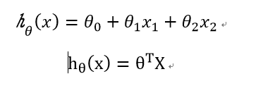
假设有X1,X2俩个特征，y为要预测值，拟合它们得关系，引入Theta参数

假设真实值与预测值存在误差ε，误差ε是独立并且具有相同的分布， 并且服从均值为0方差为θ^2 的高斯分布

对于每个样本有：

预测值与误差：




参数设置：学习率（步长）对结果影像不大，从小的时候，不行再小，一般先设置为0.01；批处理数量：32，64，128都可以，很多时候还得考虑内存和效率，一般为64.

逻辑回归理论推导

1.1逻辑回归是经典的二分类问题，决策边界是分线性的。逻辑回归采用Sigmod函数，介于（0，1）。

1.2 将函数放入Sigmoid内形成了预测函数

1.3逻辑回归，通过对数似然函数，求出损失函数l(Theate)
1.4通过求导，进行系数更新，和最后分类

逻辑回归代码实践

首先将数据导入，包含Exam1","Exam2"两个特征，"Admitted"为要预测的y,统计一下y=0和y=1的样本数据有多少，进行一个散点图的展示。

import numpy as np
import os
import time
import pandas as pd
import matplotlib.pyplot as plt
import numpy.random
from sklearn import preprocessing as pp
path="D:\Python 基础\梯度下降求解逻辑回归\data"+os.sep+"LogiReg_data.txt"
Date=pd.read_csv(path,header=None,names=["Exam1","Exam2","Admitted"])
positive=Date[Date["Admitted"]==1]
negative=Date[Date["Admitted"]==0]
fig,ax=plt.subplots()
plt.scatter(positive["Exam1"],positive["Exam2"],label="positive=1",s=30,c="red",marker="o")
plt.scatter(negative["Exam1"],negative["Exam2"],label="negative=0",s=30,c="blue")
plt.xlabel("Exam1")
plt.ylabel("Exam2")
plt.title("A student exams score")
plt.legend(loc="best")
plt.show()

简单创建模型前四部分

#1.1创建sigmoid函数
def sigmoid(z):
    return 1/(1+np.exp(-z))
#1.2创建目标函数
def model(X,Theta):
    return(sigmoid(np.dot(X,Theta.T)))
#1.3创建损失函数   
def cost(X, y, Theta):
    left = np.multiply(-y, np.log(model(X, Theta)))
    right = np.multiply(1 - y, np.log(1 - model(X, Theta)))
    return np.sum(left - right) / (len(X))
#创建梯度函数
def gradient(X, y, Theta):
    grad = np.zeros(Theta.shape)
    error = (model(X, Theta)- y).ravel()
    for j in range(len(Theta.ravel())): #for each parmeter
        term = np.multiply(error, X[:,j])
        grad[0, j] = np.sum(term) / len(X) 
    return grad

对数据进行一个简单的处理，对于Theta0,常数1最为x,所以在原始数据中插入新的一列数据，然后在对特征数据进行归一化处理，Theta数据初始化为0。

if __name__ == "__main__":
     path="D:\Python 基础\梯度下降求解逻辑回归\data"+os.sep+"LogiReg_data.txt"
     Date=pd.read_csv(path,header=None,names=["Exam1","Exam2","Admitted"])
     Date.insert(0, 'Ones', 1)#再指定的位置插入一列数据
     Date = Date.values #将DateFrame转换成数组形式
     sacle_Date = Date.copy()
     sacle_Date[:, 1:3] = pp.scale(Date[:, 1:3])#对特征数据进行归一化处理
     Theta=np.zeros([1,3])

数组的随机洗牌操作

def shuffleData(data):
    np.random.shuffle(data)
    cols = data.shape[1]
    X = data[:, 0:cols-1]
    y = data[:, cols-1:]
    return X, y

##定义三种梯度更新的策略

def stopCriterion(type, value, threshold):
    #设定三种不同的停止策略
    #1.1通过迭代次数
    #1.2通过迭代前后目标函数的差异大小
    #1.3通过迭代梯度变化大小
    if type == STOP_ITER:        return value > threshold
    elif type == STOP_COST:      return abs(value[-1]-value[-2]) < threshold
    elif type == STOP_GRAD:      return np.linalg.norm(value) < threshold

梯度更新,采用三种不同策略

def descent(data, Theta, batchSize, stopType, thresh, alpha):
    #梯度下降求解
    init_time = time.time()
    i = 0 # 迭代次数
    k = 0 # batch每次迭代的数据数量
    X, y = shuffleData(data)#重新洗牌数据
    grad=np.zeros(Theta.shape) # 计算的梯度的初始值
    costs = [cost(X,y,Theta)] # 计算损失值函数
    
    while True:
        grad = gradient(X[k:k+batchSize], y[k:k+batchSize], Theta)#计算梯度值
        k += batchSize #取batch数量个数据
        if k >= n: 
            k = 0 
            X, y = shuffleData(data) #重新洗牌
        Theta = Theta - alpha*grad # 参数更新
        costs.append(cost(X, y, Theta)) # 添加计算的损失值
        i += 1 

        if stopType == STOP_ITER:       value = i
        elif stopType == STOP_COST:     value = costs
        elif stopType == STOP_GRAD:     value = grad
        if stopCriterion(stopType, value, thresh): break

输出学习率、批量数据大小、所选择停止策略所对应的截止阈值

def runExpe(data, Theta, batchSize, stopType, thresh, alpha):
    #import pdb; pdb.set_trace();
    Theta, iter, costs, grad, dur = descent(data, Theta, batchSize, stopType, thresh, alpha)#进行梯度更新
    name = "Original" if (data[:,1]>2).sum() > 1 else "Scaled"
    name += " data - learning rate: {} - ".format(alpha)
    if batchSize==n: strDescType = "Gradient"
    elif batchSize==1:  strDescType = "Stochastic"
    else: strDescType = "Mini-batch ({})".format(batchSize)
    name += strDescType + " descent - Stop: "
    if stopType == STOP_ITER: strStop = "{} iterations".format(thresh)
    elif stopType == STOP_COST: strStop = "costs change < {}".format(thresh)
    else: strStop = "gradient norm < {}".format(thresh)
    name += strStop
    print ("***{}\nTheta: {} - Iter: {} - Last cost: {:03.2f} - Duration: {:03.2f}s".format(
        name, Theta, iter, costs[-1], dur))
    fig, ax = plt.subplots(figsize=(12,4))
    ax.plot(np.arange(len(costs)), costs, 'r')
    ax.set_xlabel('Iterations')
    ax.set_ylabel('Cost')
    ax.set_title(name.upper() + ' - Error vs. Iteration')
    return Theta

预测数据

def predict(X, Theta):
    return [1 if x >= 0.5 else 0 for x in model(X, Theta)]

整个数据的代码

import numpy as np
import os
import time
import pandas as pd
import matplotlib.pyplot as plt
import numpy.random
from sklearn import preprocessing as pp
path="D:\Python 基础\梯度下降求解逻辑回归\data"+os.sep+"LogiReg_data.txt"
Date=pd.read_csv(path,header=None,names=["Exam1","Exam2","Admitted"])
#positive=Date[Date["Admitted"]==1]
#negative=Date[Date["Admitted"]==0]
#fig,ax=plt.subplots()
#plt.scatter(positive["Exam1"],positive["Exam2"],label="positive=1",s=30,c="red",marker="o")
#plt.scatter(negative["Exam1"],negative["Exam2"],label="negative=0",s=30,c="blue")
#plt.xlabel("Exam1")
#plt.ylabel("Exam2")
#plt.title("A student exams score")
#plt.legend(loc="best")
#plt.show()

#1.1创建sigmoid函数
def sigmoid(z):
    return 1/(1+np.exp(-z))
#1.2创建目标函数
def model(X,Theta):
    return(sigmoid(np.dot(X,Theta.T)))
#1.3创建损失函数   
def cost(X, y, Theta):
    left = np.multiply(-y, np.log(model(X, Theta)))
    right = np.multiply(1 - y, np.log(1 - model(X, Theta)))
    return np.sum(left - right) / (len(X))
#创建梯度函数
def gradient(X, y, Theta):
    grad = np.zeros(Theta.shape)
    error = (model(X, Theta)- y).ravel()
    for j in range(len(Theta.ravel())): #for each parmeter
        term = np.multiply(error, X[:,j])
        grad[0, j] = np.sum(term) / len(X) 
    return grad

#洗牌
def shuffleData(data):
    np.random.shuffle(data)
    cols = data.shape[1]
    X = data[:, 0:cols-1]
    y = data[:, cols-1:]
    return X, y


def stopCriterion(type, value, threshold):
    #设定三种不同的停止策略
    #1.1通过迭代次数
    #1.2通过迭代前后目标函数的差异大小
    #1.3通过迭代梯度变化大小
    if type == STOP_ITER:        return value > threshold
    elif type == STOP_COST:      return abs(value[-1]-value[-2]) < threshold
    elif type == STOP_GRAD:      return np.linalg.norm(value) < threshold
def descent(data, Theta, batchSize, stopType, thresh, alpha):
    #梯度下降求解
    init_time = time.time()
    i = 0 # 迭代次数
    k = 0 # batch每次迭代的数据数量
    X, y = shuffleData(data)#重新洗牌数据
    grad=np.zeros(Theta.shape) # 计算的梯度的初始值
    costs = [cost(X,y,Theta)] # 计算损失值函数
    
    while True:
        grad = gradient(X[k:k+batchSize], y[k:k+batchSize], Theta)#计算梯度值
        k += batchSize #取batch数量个数据
        if k >= n: 
            k = 0 
            X, y = shuffleData(data) #重新洗牌
        Theta = Theta - alpha*grad # 参数更新
        costs.append(cost(X, y, Theta)) # 添加计算的损失值
        i += 1 

        if stopType == STOP_ITER:       value = i
        elif stopType == STOP_COST:     value = costs
        elif stopType == STOP_GRAD:     value = grad
        if stopCriterion(stopType, value, thresh): break
    
    return Theta, i-1, costs, grad, time.time() - init_time

def runExpe(data, Theta, batchSize, stopType, thresh, alpha):
    #import pdb; pdb.set_trace();
    Theta, iter, costs, grad, dur = descent(data, Theta, batchSize, stopType, thresh, alpha)#进行梯度更新
    
    
    name = "Original" if (data[:,1]>2).sum() > 1 else "Scaled"
    name += " data - learning rate: {} - ".format(alpha)
    if batchSize==n: strDescType = "Gradient"
    elif batchSize==1:  strDescType = "Stochastic"
    else: strDescType = "Mini-batch ({})".format(batchSize)
    name += strDescType + " descent - Stop: "
    if stopType == STOP_ITER: strStop = "{} iterations".format(thresh)
    elif stopType == STOP_COST: strStop = "costs change < {}".format(thresh)
    else: strStop = "gradient norm < {}".format(thresh)
    name += strStop
    print ("***{}\nTheta: {} - Iter: {} - Last cost: {:03.2f} - Duration: {:03.2f}s".format(
        name, Theta, iter, costs[-1], dur))
    fig, ax = plt.subplots(figsize=(12,4))
    ax.plot(np.arange(len(costs)), costs, 'r')
    ax.set_xlabel('Iterations')
    ax.set_ylabel('Cost')
    ax.set_title(name.upper() + ' - Error vs. Iteration')
    
    return Theta
#设定阈值
def predict(X, Theta):
    return [1 if x >= 0.5 else 0 for x in model(X, Theta)]

if __name__ == "__main__":
     path="D:\Python 基础\梯度下降求解逻辑回归\data"+os.sep+"LogiReg_data.txt"
     Date=pd.read_csv(path,header=None,names=["Exam1","Exam2","Admitted"])
     Date.insert(0, 'Ones', 1)#再指定的位置插入一列数据
     Date = Date.values #将DateFrame转换成数组形式
     sacle_Date = Date.copy()
     sacle_Date[:, 1:3] = pp.scale(Date[:, 1:3])#对特征数据进行归一化处理
     Theta=np.zeros([1,3])
     STOP_ITER = 0
     STOP_COST = 1
     STOP_GRAD = 2
     n=100
     print(runExpe(sacle_Date, Theta, 16, STOP_GRAD, thresh=0.002*2, alpha=0.001))
     scaled_X = sacle_Date[:, :3]
     y = sacle_Date[:, 3]
     predictions = predict(scaled_X, runExpe(sacle_Date, Theta, 16, STOP_GRAD, thresh=0.002*2, alpha=0.001))
     correct = [1 if ((a == 1 and b == 1) or (a == 0 and b == 0)) else 0 for (a, b) in zip(predictions, y)]
     accuracy = (sum(map(int, correct)) % len(correct))
     print ('accuracy = {0}%'.format(accuracy))#输出精度