逻辑斯谛回归--Python代码实现

原文出处

本文在原文的基础上增加仅一些个人理解

前言

上一篇文章中，已经说明在逻辑斯谛回归模型中就是利用极大似然估计，来求出参数$\displaystyle \omega$，然后根据输入的$\displaystyle x$，利用公式来预测$\displaystyle y$

在本文中，当求出$\displaystyle \omega$后，不再利用$\displaystyle P(Y=1|x)=\dfrac {\exp \left( wx\right) }{1+\exp \left( wx\right) }$以及$\displaystyle P(Y=0|x)=\dfrac {1}{1+\exp \left( wx\right) }$两个公式分别计算出$\displaystyle Y=0$以及$\displaystyle Y=1$的概率，而是用一个$\displaystyle sigmoid$函数来计算概率，当计算出的值接近于1时，也即是$\displaystyle Y=1$，当计算出的值接近于0时，也即是$\displaystyle Y=0$

正文

生成数据

本文中将使用模拟数据，我们可以从多维正态分布中取样

import numpy as np
import matplotlib.pyplot as plt
%matplotlib inline

np.random.seed(12)
num_observations = 5000

x1 = np.random.multivariate_normal([0, 0], [[1, .75],[.75, 1]], num_observations)
x2 = np.random.multivariate_normal([1, 4], [[1, .75],[.75, 1]], num_observations)

simulated_separableish_features = np.vstack((x1, x2)).astype(np.float32)
simulated_labels = np.hstack((np.zeros(num_observations),
                              np.ones(num_observations)))

正态分布

$$x\sim N\left(\sigma,\mu ^{2}\right)$$
可以看出，对于一个正态分布有两个重要的参数 期望和方差
[1] $\displaystyle np.random.multivariate\_normal$ 参数含义
观测生成的数据

plt.figure(figsize=(12,8))
plt.scatter(simulated_separableish_features[:, 0], simulated_separableish_features[:, 1],
            c = simulated_labels, alpha = .4)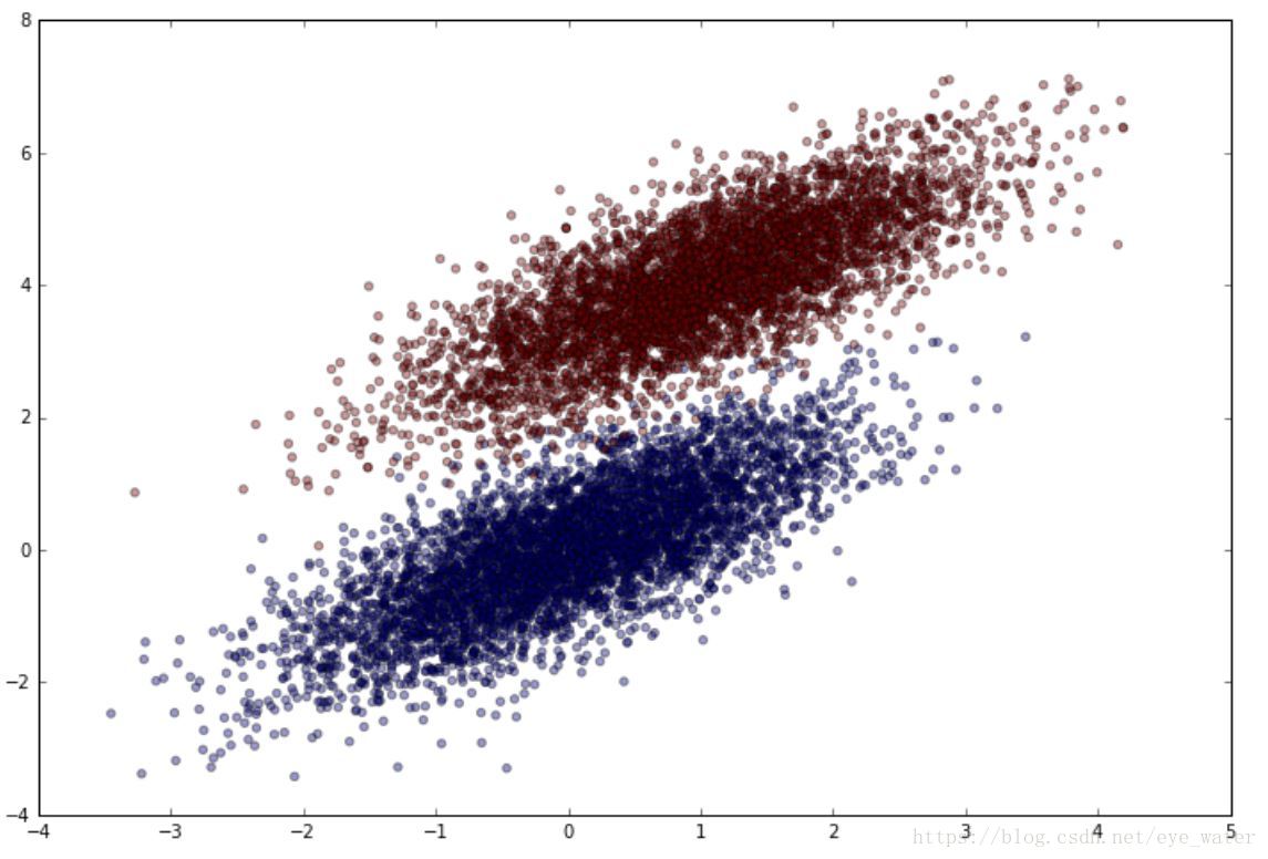

选择预测函数

一般的线性模型都会使用联系函数将线性模型与预测值联系起来，在逻辑斯谛回归模型中，使用$\displaystyle sigmoid$函数作为联系函数

def sigmoid(scores):
    return 1 / (1 + np.exp(-scores))

极大似然估计

为了最大化似然函数，我们需要似然函数的公式以及似然函数的梯度。幸运的是， 对于二分类问题来说似然函数可以转变为对数似然函数。在极大似然估计中，我们可以不用影响权重参数评估来达到我们的目的，因为对数变换是单调的。

对数似然计算

可以把对数似然函数看作所有训练数据的和
公式：

$$ll=\sum ^{n}_{i=1}y_{i}\beta ^{T}x_{i}-\log \left( 1+\beta ^{T}x_{i}\right)$$
$\displaystyle y$是目标分类(0或1)， $\displaystyle xi$是输入数据， $\displaystyle \beta$是权重向量

梯度计算

我们需要一个计算对数似然函数的公式，可以对上面的公式进行求导并再形成一个矩阵

$$\nabla ll=X^{T}(Y-Predictions)$$

建立逻辑斯谛回归函数

$\displaystyle Slope \ and \ Intercept$

def logistic_regression(features, target, num_steps, learning_rate, add_intercept = False):
    if add_intercept:
        intercept = np.ones((features.shape[0], 1))
        features = np.hstack((intercept, features))

    weights = np.zeros(features.shape[1])

    for step in xrange(num_steps):
        scores = np.dot(features, weights)
        predictions = sigmoid(scores)

        # Update weights with gradient
        output_error_signal = target - predictions
        gradient = np.dot(features.T, output_error_signal)
        weights += learning_rate * gradient

        # Print log-likelihood every so often
        if step % 10000 == 0:
            print log_likelihood(features, target, weights)

    return weights

关于for循环
可以与梯度下降法做一个比较

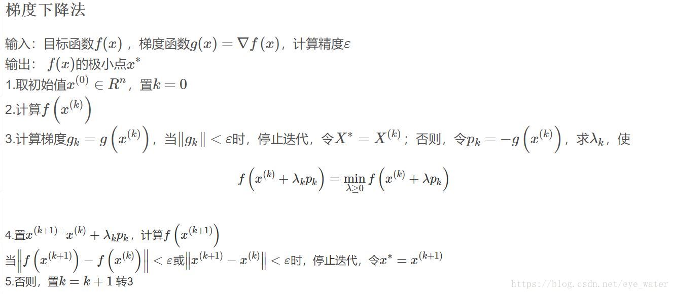
可以看到for循环里面的步骤与梯度下降法大致一样
不同的是，相比于梯度下降法，for循环中我们用定值learning_rate来代替$\displaystyle \lambda _{k}$，并且我们并没有判定当函数增长幅度十分小时是否应当退出循环
运行Logistic Regression

weights = logistic_regression(simulated_separableish_features, simulated_labels,
                     num_steps = 300000, learning_rate = 5e-5, add_intercept=True)

输出

-4346.26477915
-148.706722768
-142.964936231
-141.545303072
-141.060319659
-140.870315859
-140.790259128
...
-140.725421355

与Sk-Learn 中的 LogisticRegression 做比较

我们并不知道我们自己的算法计算出的权重值是否正确，但是我们知道Sk-Learn 中的 LogisticRegression算法是正确的，因此把我们自己计算出的权重值与Sk-Learn 中的 LogisticRegression计算出的权重值进行比较即可

from sklearn.linear_model import LogisticRegression

clf = LogisticRegression(fit_intercept=True, C = 1e15)
clf.fit(simulated_separableish_features, simulated_labels)
print(clf.intercept_, clf.coef_)
print(weights)

输出

[-13.99400797] [[-5.02712572  8.23286799]]
[-14.09225541  -5.05899648   8.28955762]

看起来结果不错，但是如果我们进行更多次的循环以及给出一个足够小的learning_rate我们会得到一个更好的结果

为什么?

当我们极大化对数似然函数时，我们用的是梯度上升法（和梯度下降法差不多，差别仅仅是一个负号）
梯度下降法有一个性质，当目标函数是凸函数时，梯度下降法的解是最优解
梯度上升法和梯度下降法仅仅相差一个负号，因此可以得出梯度上升法的性质：当目标函数是凹函数时，梯度下降法的解是最优解
[2]$\displaystyle 李航.附录A \ 梯度下降法.统计学习方法.2012$

精确度

最后，我们要利用求出来的权重值$\displaystyle \omega$通过$\displaystyle sigmoid$函数来计算分类值，就像前言中提到的那样，当计算出的值接近于1时，也即是$\displaystyle Y=1$，当计算出的值接近于0时，也即是$\displaystyle Y=0$，最后我们计算精确度

data_with_intercept = np.hstack((np.ones((simulated_separableish_features.shape[0], 1)),
                                simulated_separableish_features))
final_scores = np.dot(data_with_intercept, weights)
preds = np.round(sigmoid(final_scores))
print('Accuracy from scratch: {0}'.format((preds == simulated_labels).sum().astype(float) / len(preds)))
print('Accuracy from sk-learn: {0}'.format(clf.score(simulated_separableish_features, simulated_labels)))

输出：

Accuracy from scratch: 0.9948
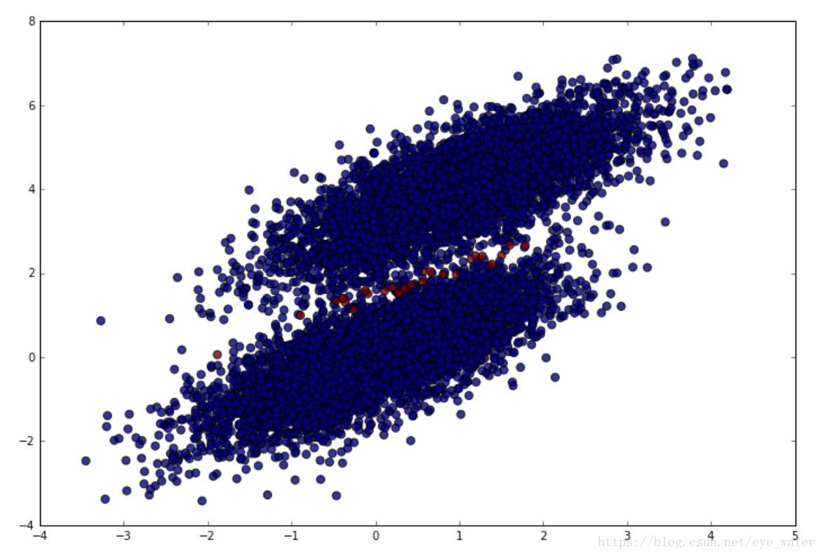
Accuracy from sk-learn: 0.9948

我们可以将我们估算错误的值显示在两个正确分类的中间，红色是估算错的，蓝色是估算对的

plt.figure(figsize = (12, 8))
plt.scatter(simulated_separableish_features[:, 0], simulated_separableish_features[:, 1],
            c = preds == simulated_labels - 1, alpha = .8, s = 50)