Catalog

完整代码

import requests, re, pandas as pd, numpy as np, matplotlib.pyplot as mp
# 从网络下载数据
def download():
    url = 'https://blog.csdn.net/Yellow_python/article/details/81240395'
    header = {'User-Agent': 'Opera/8.0 (Windows NT 5.1; U; en)'}
    r = requests.get(url, headers=header)
    data = re.findall('<pre><code>([\s\S]+?)</code></pre>', r.text)[0].strip()
    df = pd.DataFrame([i.split(',') for i in data.split()], columns=['x1', 'x2', 'y'])
    df['x1'] = pd.to_numeric(df['x1'])
    df['x2'] = pd.to_numeric(df['x2'])
    df['y'] = pd.to_numeric(df['y'])  # 正例和负例
    return df
# 数据处理
def handle(df):
    # 增加一列，并转换成矩阵，用以矩阵相乘
    df.insert(0, 'one', 1)
    matrix = df.as_matrix()
    # 纵向切分
    X = matrix[:, 0:-1]  # Ones, x1, x2
    y = matrix[:, -1:]  # y
    return X, y
# sigmoid函数
sigmoid = lambda x: 1 / (1 + np.exp(-x))
# 梯度上升
def gradient_ascent(X, y):
    m = X.shape[1]
    theta = np.mat([[1]] * m)  # 初始化回归系数
    for i in range(99, 999999):
        alpha = 1 / i  # 步长（先大后小）
        h = sigmoid(X * theta)
        theta = theta + alpha * X.transpose() * (y - h)  # 最终梯度上升迭代公式
    return theta
# 数据可视化
def visualize(df, theta):
    # 散点图：正例和负例
    positive = df[df['y'] == 1]
    negative = df[df['y'] == 0]
    mp.scatter(positive['x1'], positive['x2'], c='g', marker='o', label='positive')
    mp.scatter(negative['x1'], negative['x2'], c='r', marker='x', label='negative')
    # 折线图：决策边界
    min_x1 = df['x1'].min()
    max_x1 = df['x1'].max()
    x = np.arange(min_x1, max_x1, 2)
    y = (-theta[0, 0] - theta[1, 0] * x) / theta[2, 0]  # 边界函数
    mp.plot(x, y, label='boundary')
    # 展示图形
    mp.legend()
    mp.show()
# 主函数
def main():
    df = download()
    X, y = handle(df)
    theta = gradient_ascent(X, y)
    print(theta)
    visualize(df, theta)
# 执行
if __name__=='__main__':
    main()

这里写图片描述

步骤

1、数据读取（直接复制即可）

import requests, re, pandas as pd
def download():
    url = 'https://blog.csdn.net/Yellow_python/article/details/81240395'
    header = {'User-Agent': 'Opera/8.0 (Windows NT 5.1; U; en)'}
    r = requests.get(url, headers=header)
    data = re.findall('<pre><code>([\s\S]+?)</code></pre>', r.text)[0].strip()
    df = pd.DataFrame([i.split(',') for i in data.split()], columns=['x1', 'x2', 'y'])
    df['x1'] = pd.to_numeric(df['x1'])
    df['x2'] = pd.to_numeric(df['x2'])
    df['y'] = pd.to_numeric(df['y'])
    return df

2、数据预处理

def handle(df):
    # 增加一列，并转换成矩阵，用以矩阵相乘
    df.insert(0, 'one', 1)
    matrix = df.as_matrix()
    # 纵向切分
    X = matrix[:, 0:-1]  # Ones, x1, x2
    y = matrix[:, -1]  # y
    return X, y

3、Sigmoid函数

import numpy as np
import matplotlib.pyplot as mp
sigmoid = lambda x: 1 / (1 + np.exp(-x))  # sigmoid函数
x = np.linspace(-8, 8, 65)
mp.plot(x, sigmoid(x), label=r'$S(x)=\frac{1}{1+e^{-x}}$')
mp.legend()
mp.show()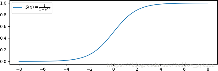

这里写图片描述

Sigmoid函数可将变量映射到 $(0,1)$

g (z) = \frac{1}{1 + e^{- z}}

$g(z) = \frac {1} {1+e^{-z}}$

θ^{T} x = [\begin{matrix} θ_{1} & θ_{2} & \dots & θ_{m} \end{matrix}] [\begin{matrix} x_{1} \\ x_{2} \\ ⋮ \\ x_{m} \end{matrix}]

$\theta^Tx = \begin{bmatrix} \theta_1 & \theta_2 & \ldots & \theta_m \end{bmatrix} \begin{bmatrix} x_1 \\ x_2 \\ \vdots \\ x_m \end{bmatrix}$

h_{θ} (x) = g (θ^{T} x) = \frac{1}{1 + e^{- θ^{T} x}}

$h_\theta (x) = g(\theta^Tx) = \frac {1} {1+e^{-\theta^Tx}}$

扫描二维码关注公众号，回复： 2596239 查看本文章

4、梯度上升

4.1、梯度上升迭代公式

先了解 Python梯度上升算法，然后根据其原理，获得最终公式
$θ := θ + α X^{T} (y - h)$ $\theta := \theta + \alpha X^T (y - h)$: 具体指代：

θ = [\begin{matrix} θ_{1} \\ θ_{2} \\ ⋮ \\ θ_{m} \end{matrix}]

$\theta = \begin{bmatrix} \theta_1 \\ \theta_2 \\ \vdots \\ \theta_m \end{bmatrix}$

X = (\begin{matrix} 1 & x_{12} & x_{13} & \dots & x_{1 m} \\ 1 & x_{22} & x_{33} & \dots & x_{2 m} \\ ⋮ & ⋮ & ⋮ & ⋱ & ⋮ \\ 1 & x_{n 2} & x_{n 3} & \dots & x_{n m} \end{matrix})

$X = \begin{pmatrix} 1 & x_{12} & x_{13} & \cdots & x_{1m} \\ 1 & x_{22} & x_{33} & \cdots & x_{2m} \\ \vdots & \vdots & \vdots & \ddots & \vdots \\ 1 & x_{n2} & x_{n3} & \cdots & x_{nm} \\ \end{pmatrix}$

y = [\begin{matrix} y_{1} \\ y_{2} \\ ⋮ \\ y_{n} \end{matrix}]

$y = \begin{bmatrix} y_1 \\ y_2 \\ \vdots \\ y_n \end{bmatrix}$

h = S i g m o i d (X θ) = \frac{1}{1 + e^{- (X θ)}}

$h = Sigmoid(X \theta) = \frac {1} {1+e^{-(X \theta)}}$

4.2、代码实现

4.2.1、龟速版

每次迭代一小步，迭代足够多的次数

def gradient_ascent(X, y):
    m = X.shape[1]
    theta = np.mat([[1]] * m)  # 初始化回归系数
    alpha = 0.00001  # 步长
    cycles = 999999  # 迭代次数
    for i in range(cycles):
        h = sigmoid(X * theta)
        theta = theta + alpha * X.transpose() * (y - h)  # 最终梯度上升迭代公式
    return theta

4.2.2、改进版

前期大步迭代，后期小步迭代

def gradient_ascent(X, y):
    m = X.shape[1]
    theta = np.mat([[1]] * m)
    for i in range(99, 999999):
        alpha = 1 / i  # 步长（先大后小）
        h = sigmoid(X * theta)
        theta = theta + alpha * X.transpose() * (y - h)
    return theta

附录

补充

相关知识链接：

翻译：

alpha: 希腊字母的第1个字母： $\alpha$
theta: 希腊字母的第8个字母： $\theta$
presision: 精度
gradient ascent: 梯度上升

数据源

34.62365962451697,78.0246928153624,0
30.28671076822607,43.89499752400101,0
35.84740876993872,72.90219802708364,0
60.18259938620976,86.30855209546826,1
79.0327360507101,75.3443764369103,1
45.08327747668339,56.3163717815305,0
61.10666453684766,96.51142588489624,1
75.02474556738889,46.55401354116538,1
76.09878670226257,87.42056971926803,1
84.43281996120035,43.53339331072109,1
95.86155507093572,38.22527805795094,0
75.01365838958247,30.60326323428011,0
82.30705337399482,76.48196330235604,1
69.36458875970939,97.71869196188608,1
39.53833914367223,76.03681085115882,0
53.9710521485623,89.20735013750205,1
69.07014406283025,52.74046973016765,1
67.94685547711617,46.67857410673128,0
70.66150955499435,92.92713789364831,1
76.97878372747498,47.57596364975532,1
67.37202754570876,42.83843832029179,0
89.67677575072079,65.79936592745237,1
50.534788289883,48.85581152764205,0
34.21206097786789,44.20952859866288,0
77.9240914545704,68.9723599933059,1
62.27101367004632,69.95445795447587,1
80.1901807509566,44.82162893218353,1
93.114388797442,38.80067033713209,0
61.83020602312595,50.25610789244621,0
38.78580379679423,64.99568095539578,0
61.379289447425,72.80788731317097,1
85.40451939411645,57.05198397627122,1
52.10797973193984,63.12762376881715,0
52.04540476831827,69.43286012045222,1
40.23689373545111,71.16774802184875,0
54.63510555424817,52.21388588061123,0
33.91550010906887,98.86943574220611,0
64.17698887494485,80.90806058670817,1
74.78925295941542,41.57341522824434,0
34.1836400264419,75.2377203360134,0
83.90239366249155,56.30804621605327,1
51.54772026906181,46.85629026349976,0
94.44336776917852,65.56892160559052,1
82.36875375713919,40.61825515970618,0
51.04775177128865,45.82270145776001,0
62.22267576120188,52.06099194836679,0
77.19303492601364,70.45820000180959,1
97.77159928000232,86.7278223300282,1
62.07306379667647,96.76882412413983,1
91.56497449807442,88.69629254546599,1
79.94481794066932,74.16311935043758,1
99.2725269292572,60.99903099844988,1
90.54671411399852,43.39060180650027,1
34.52451385320009,60.39634245837173,0
50.2864961189907,49.80453881323059,0
49.58667721632031,59.80895099453265,0
97.64563396007767,68.86157272420604,1
32.57720016809309,95.59854761387875,0
74.24869136721598,69.82457122657193,1
71.79646205863379,78.45356224515052,1
75.3956114656803,85.75993667331619,1
35.28611281526193,47.02051394723416,0
56.25381749711624,39.26147251058019,0
30.05882244669796,49.59297386723685,0
44.66826172480893,66.45008614558913,0
66.56089447242954,41.09209807936973,0
40.45755098375164,97.53518548909936,1
49.07256321908844,51.88321182073966,0
80.27957401466998,92.11606081344084,1
66.74671856944039,60.99139402740988,1
32.72283304060323,43.30717306430063,0
64.0393204150601,78.03168802018232,1
72.34649422579923,96.22759296761404,1
60.45788573918959,73.09499809758037,1
58.84095621726802,75.85844831279042,1
99.82785779692128,72.36925193383885,1
47.26426910848174,88.47586499559782,1
50.45815980285988,75.80985952982456,1
60.45555629271532,42.50840943572217,0
82.22666157785568,42.71987853716458,0
88.9138964166533,69.80378889835472,1
94.83450672430196,45.69430680250754,1
67.31925746917527,66.58935317747915,1
57.23870631569862,59.51428198012956,1
80.36675600171273,90.96014789746954,1
68.46852178591112,85.59430710452014,1
42.0754545384731,78.84478600148043,0
75.47770200533905,90.42453899753964,1
78.63542434898018,96.64742716885644,1
52.34800398794107,60.76950525602592,0
94.09433112516793,77.15910509073893,1
90.44855097096364,87.50879176484702,1
55.48216114069585,35.57070347228866,0
74.49269241843041,84.84513684930135,1
89.84580670720979,45.35828361091658,1
83.48916274498238,48.38028579728175,1
42.2617008099817,87.10385094025457,1
99.31500880510394,68.77540947206617,1
55.34001756003703,64.9319380069486,1
74.77589300092767,89.52981289513276,1

Python【逻辑回归】简洁代码