What is this article about?

This article provides an overview of the main models available for modelling time series and forecasting their evolution. The models were developed in R and Python. The related code is available here.

Time series forecasting is a hot topic which has many possible applications, such as stock prices forecasting, weather forecasting, business planning, resources allocation and many others. Even though forecasting can be considered as a subset of supervised regression problems, some specific tools are necessary due to the temporal nature of observations.

What is a time series?

A time series is usually modelled through a stochastic process Y(t), i.e. a sequence of random variables. In a forecasting setting we find ourselves at time t and we are interested in estimating Y(t+h), using only information available at time t.

How to validate and test a time series model?

Due to the temporal dependencies in time series data, we cannot rely on usual validation techniques. To avoid biased evaluations we must ensure that training sets contains observations that occurred prior to the ones in validation sets.

A possible way to overcome this problem is to use a sliding window, as described here. This procedure is called time series cross validation and it is summarised in the following picture, in which the blue points represents the training sets in each “fold” and the red points represent the corresponding validation sets.

Time series cross-validation. Credits to Rob J Hyndman

If we are interested in forecasting the next n time steps, we can apply the cross validation procedure for 1,2,…,n steps ahead. In this way we can also compare the goodness of the forecasts for different time horizons.

Once we have chosen the best model, we can fit it on the entire training set and evaluate its performance on a separate test set subsequent in time. The performance estimate can be done by using the same sliding window technique used for cross validation, but without re-estimating the model parameters.

Short data exploration

In the next section we will apply different forecasting models to predict the evolution of the industrial production index which quantifies the electrical equipment manufactured in the Euro area.

The data can be easily downloaded through the fpp2 package in R. To make the data available outside R you can simply run the following code in a R environment.

library(fpp2)
write.csv(elecequip,file = “elecequip.csv”,row.names = FALSE)

The dataset corresponds to monthly manufacture of electrical equipment (computer, electronic and optical products) in the Euro area (17 countries) in the period January 1996-March 2012. We keep the last 2 years for testing purposes.

The time series has a peak at the end of 2000 and another one during 2007. The huge decrease that we observe at the end of 2008 is probably due to the global financial crisis which occurred during that year.

There seems to be a yearly seasonal pattern. To better visualise this, we show data for each year separately in both original and polar coordinates.

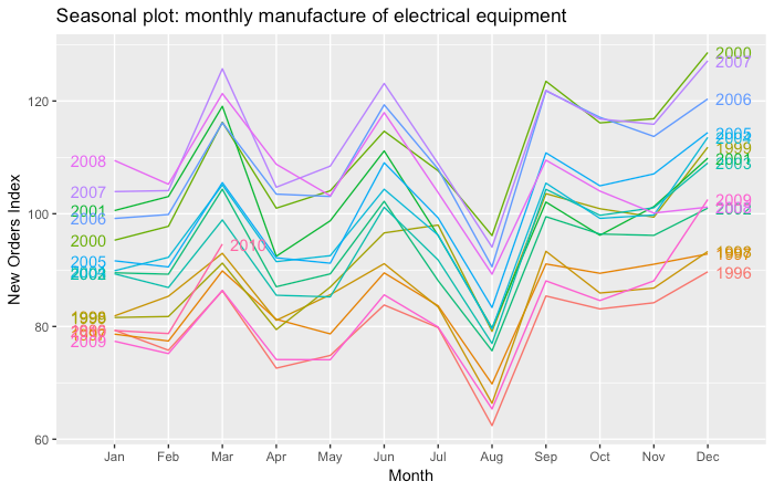
We observe a strong seasonal pattern. In particular there is a huge decline in production in August due to the summer holidays.

Time series forecasting models

We will consider the following models:

Naïve, SNaïve
Seasonal decomposition (+ any model)
Exponential smoothing
ARIMA, SARIMA
GARCH
Dynamic linear models
TBATS
Prophet
NNETAR
LSTM

We are interested in forecasting 12 months of the industrial production index. Therefore, given data up to time t, we would like to predict the values taken by the index at times t+1,…,t+12.

We will use the Mean Absolute Error (MAE) to assess the performance of the models.

1) Naïve, SNaïve

In the Naïve model, the forecasts for every horizon correspond to the last observed value.

Ŷ(t+h|t) = Y(t)

This kind of forecast assumes that the stochastic model generating the time series is a random walk.

An extension of the Naïve model is given by the SNaïve (Seasonal Naïve) model. Assuming that the time series has a seasonal component and that the period of the seasonality is T, the forecasts given by the SNaïve model are given by:

Ŷ(t+h|t) = Y(t+h-T)

Therefore the forecasts for the following T time steps are equal to the previous T time steps. In our application, the SNaïve forecast for the next year is equal to the last year’s observations.

These models are often used as benchmark models. The following plots show the predictions obtained with the two models for the year 2007.

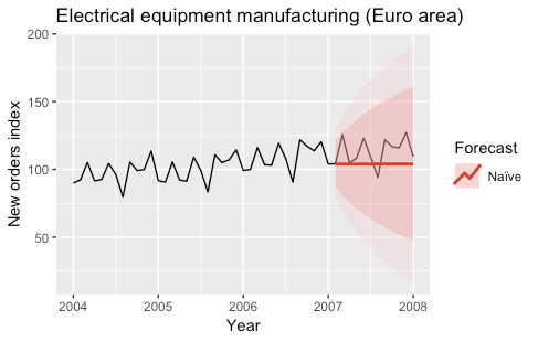
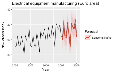
The models were fitted by using the naive and snaive functions of the forecast R package.

2) Seasonal decomposition (+ any model)

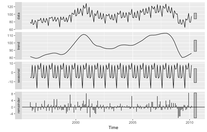
If data shows some seasonality (e.g. daily, weekly, quarterly, yearly) it may be useful to decompose the original time series into the sum of three components:

Y(t) = S(t) + T(t) + R(t)

where S(t) is the seasonal component, T(t) is the trend-cycle component, and R(t) is the remainder component.

There exists several techniques to estimate such a decomposition. The most basic one is called classical decomposition and it consists in:

Estimating trend T(t) through a rolling mean
Computing S(t) as the average detrended series Y(t)-T(t) for each season (e.g. for each month)
Computing the remainder series as R(t)=Y(t)-T(t)-S(t)

The classical decomposition has been extended in several ways. Its extensions allow to:

have a non-constant seasonality
compute initial and last values of the decomposition
avoid over-smoothing

To get an overview of time series decomposition methods you can click here. We will take advantage of the STL decomposition, which is known to be versatile and robust.

STL decomposition on industrial production index data

One way to use the decomposition for forecasting purposes is the following:

Decompose the training time series with some decomposition algorithm (e.g. STL): Y(t)= S(t)+T(t)+R(t).
Compute the seasonally adjusted time series Y(t)-S(t). Use any model you like to forecast the evolution of the seasonally adjusted time series.
Add to the forecasts the seasonality of the last time period in the time series (in our case, the fitted S(t) for last year).

In the following picture we show the seasonally adjusted industrial production index time series.

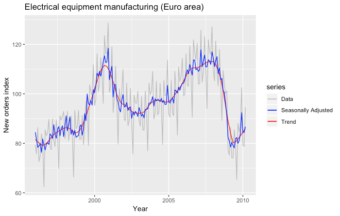
The following plot shows the predictions obtained for the year 2007 by using the STL decomposition and the naïve model to fit the seasonally adjusted time series.

The decomposition was fitted by using the stl function of the stats R package.

3) Exponential smoothing

Exponential smoothing is one of the most successful classical forecasting methods. In its basic form it is called simple exponential smoothing and its forecasts are given by:

Ŷ(t+h|t) = ⍺y(t) + ⍺(1-⍺)y(t-1) + ⍺(1-⍺)²y(t-2) + …

with 0<⍺<1.

We can see that forecasts are equal to a weighted average of past observations and the corresponding weights decrease exponentially as we go back in time.

Several extensions of the simple exponential smoothing have been proposed in order to include trend or damped trend and seasonality. The exponential smoothing family is composed of 9 models which are fully described here.

The following plots show the predictions obtained for the year 2007 by using exponential smoothing models (automatically selected) to fit both the original and the seasonally adjusted time series.

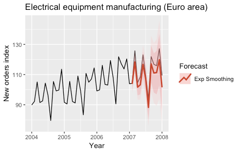
The models were fitted by using the ets function of the forecast R package.

4) ARIMA, SARIMA

As for exponential smoothing, also ARIMA models are among the most widely used approaches for time series forecasting. The name is an acronym for AutoRegressive Integrated Moving Average.

In an AutoRegressive model the forecasts correspond to a linear combination of past values of the variable. In a Moving Average model the forecasts correspond to a linear combination of past forecast errors.

Basically, the ARIMA models combine these two approaches. Since they require the time series to be stationary, differencing (Integrating) the time series may be a necessary step, i.e. considering the time series of the differences instead of the original one.

The SARIMA model (Seasonal ARIMA) extends the ARIMA by adding a linear combination of seasonal past values and/or forecast errors.

For a complete introduction to ARIMA and SARIMA models, click here.

The following plots show the predictions obtained for the year 2007 by using a SARIMA model and an ARIMA model on the seasonally adjusted time series.

The models were fitted by using the auto.arima and Arima functions of the forecast R package.

5) GARCH

The previous models assumed that the error terms in the stochastic processes generating the time series were heteroskedastic, i.e. with constant variance.

Instead, the GARCH model assumes that the variance of the error terms follows an AutoRegressive Moving Average (ARMA) process, therefore allowing it to change in time. It is particularly useful for modelling financial time series whose volatility changes across time. The name is an acronym for Generalised Autoregressive Conditional Heteroskedasticity.

Usually an ARMA process is assumed for the mean as well. For a complete introduction to GARCH models you can click here and here.

The following plots show the predictions obtained for the year 2007 by using a GARCH model to fit the seasonally adjusted time series.

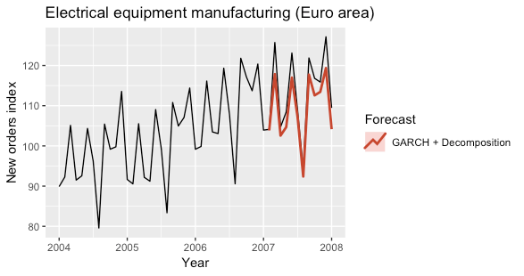
The model was fitted by using the ugarchfitfunction of the rugarch R package.

6) Dynamic linear models

Dynamic linear models represent another class of models for time series forecasting. The idea is that at each time t these models correspond to a linear model, but the regression coefficients change in time. An example of dynamic linear model is given below.

y(t) = ⍺(t) + tβ(t) + w(t)

⍺(t) = ⍺(t-1) + m(t)

β(t) = β(t-1) + r(t)

w(t)~N(0,W) , m(t)~N(0,M) , r(t)~N(0,R)

In the previous model the coefficients ⍺(t) and β(t) follow a random walk process.

Dynamic linear models can be naturally modelled in a Bayesian framework; however maximum likelihood estimation techniques are still available. For a complete overview of dynamic linear models, click here.

The following plot shows the predictions obtained for the year 2007 by using a dynamic linear model to fit the seasonally adjusted time series. Due to heavy computational costs I had to keep the model extremely simple which resulted in poor forecasts.

The model was fitted by using the dlmMLEfunction of the dlm R package.

7) TBATS

The TBATS model is a forecasting model based on exponential smoothing. The name is an acronym for Trigonometric, Box-Cox transform, ARMA errors, Trend and Seasonal components.

The main feature of TBATS model is its capability to deal with multiple seasonalities by modelling each seasonality with a trigonometric representation based on Fourier series. A classic example of complex seasonality is given by daily observations of sales volumes which often have both weekly and yearly seasonality.

For a complete introduction of TBATS model, click here.

The following plot shows the predictions obtained for the year 2007 by using a TBATS model to fit the time series.

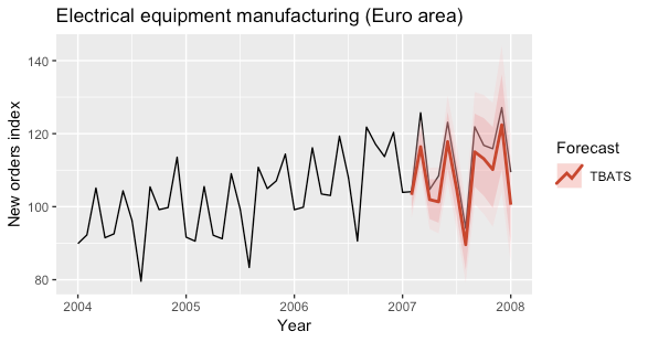
The model was fitted by using the tbats function of the forecast R package.

8) Prophet

Prophet is another forecasting model which allows to deal with multiple seasonalities. It is an open source software released by Facebook’s Core Data Science team.

The prophet model assumes that the the time series can be decomposed as follows:

y(t) = g(t) + s(t) + h(t) + ε(t)

The three terms g(t), s(t) and h(t) correspond respectively to trend, seasonality and holiday. The last term is the error term.

The model fitting is framed as a curve-fitting exercise, therefore it does not explicitly take into account the temporal dependence structure in the data. This also allows to have irregularly spaced observations.

There are two options for trend time series: a saturating growth model, and a piecewise linear model. The multi-period seasonality model relies on Fourier series. The effect of known and custom holydays can be easily incorporated into the model.

The prophet model is inserted in a Bayesian framework and it allows to make full posterior inference to include model parameter uncertainty in the forecast uncertainty.

For a complete introduction to Prophet model, click here.

The following plot shows the predictions obtained for the year 2007 by using a Prophet model to fit the time series.

The model was fitted by using the prophet function of the prophet R package.

9) NNETAR

The NNETAR model is a fully connected neural network. The acronym stands for Neural NETwork AutoRegression.

The NNETAR model takes in input the last elements of the sequence up to time t and outputs the forecasted value at time t+1. To perform multi-steps forecasts the network is applied iteratively.

In presence of seasonality, the input may include also the seasonally lagged time series. For a complete introduction to NNETAR models, click here.

The following plots show the predictions obtained for the year 2007 obtained by using a NNETAR model with seasonally lagged input and a NNETAR model on the seasonally adjusted time series.

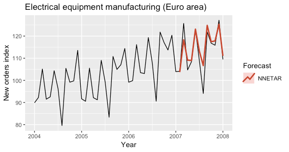
The models were fitted by using the nnetar function of the forecast R package.

10) LSTM

LSTM models can be used to forecast time series (as well as other Recurrent Neural Networks). LSTM is an acronym that stands for Long-Short Term Memories.

The state of a LSTM network is represented through a state space vector. This technique allows to keep tracks of dependencies of new observations with past ones (even very far ones).

LSTMs may benefit from transfer learning techniques even when applied to standard time series, as shown here. However, they are mostly used with unstructured data (e.g. audio, text, video).

For a complete introduction on using LSTM to forecast time series, click here.

The following plot shows the predictions for the first year in the test set obtained by fitting a LSTM model on the seasonally adjusted time series.

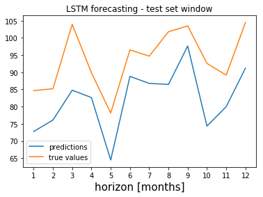
The model was fitted by using the Keras framework in Python.

Evaluation

We performed model selection through the cross-validation procedure described previously. We didn’t compute it for dynamic linear models and LSTM models due to their high computational cost and poor performance.

In the following picture we show the cross-validated MAE for each model and for each time horizon.

We can see that, for time horizons greater than 4, the NNETAR model on the seasonally adjusted data performed better than the others. Let’s check the overall MAE computed by averaging over different time horizons.

Cross-validated MAE

The NNETAR model on the seasonally adjusted data was the best model for this application since it corresponded to the lowest cross-validated MAE.

To get an unbiased estimation of the best model performance, we computed the MAE on the test set, obtaining an estimate equal to 5,24. In the following picture we can see the MAE estimated on the test set for each time horizon.

How to further improve performance

Other techniques to increase models performance could be:

Using different models for different time horizons
Combining multiple forecasts (e.g. considering the average prediction)
Bootstrap Aggregating

The last technique can be summarised as follows:

Decompose the original time series (e.g. by using STL)
Generate a set of similar time series by randomly shuffling chunks of the Remainder component
Fit a model on each time series
Average forecasts of every model

For a complete introduction to Bootstrap Aggregating, click here.

Other models

Other models not included in this list are for instance:

Any standard regression model, taking time as input (and/or other features)
Encoder Decoder models, which are tipically used in NLP tasks (e.g. translation)
Wavenet and other Attention Networks, which are tipically applied to unstructured data (e.g. Text-to-Speech)

Final remarks

The goal of this project wasn’t to fit the best possible forecasting model for industrial production index, but to give an overview of forecasting models. In a real world application a lot of time should be spent on preprocessing, feature engineering and feature selection.

Most of the previously described models allow to easily incorporate time varying predictors. These could be extracted from the same time series or could correspond to external predictors (e.g. the time series of another index). In the latter case we should pay attention to not use information from the future, which could be satisfied by forecasting the predictors or by using their lagged versions.

An overview of time series forecasting models