【论文精读】一石二鸟：Series Saliency for Accurate and Interpretable Multivariate Time Series Forecasting

Two Birds with One Stone: Series Saliency for Accurate and Interpretable Multivariate Time Series Forecasting

Abstract

It is important yet challenging to perform accurate and interpretable time series forecasting. Though deep learning methods can boost the forecasting accuracy, they often sacrifice interpretability. In this paper, we present a new scheme of series saliency to boost both accuracy and interpretability. By extracting series images from sliding windows of the time series, we design series saliency as a mixup strategy with a learnable mask between the series images and their perturbed versions. Series saliency is model agnostic and performs as an adaptive data augmentation method for training deep models. Moreover, by slightly changing the objective, we optimize series saliency to find a mask for interpretable forecasting in both feature and time dimensions. Experimental results on several real datasets demonstrate that series saliency is effective to produce accurate time-series forecasting results as well as generate temporal interpretations

准确、可解释的时间序列预测是一项重要而又具有挑战性的工作。尽管深度学习方法可以提高预测的准确性，但它们往往牺牲了可解释性。在本文中，我们提出了一个新的序列显著性（series saliency）方案，以提高准确性和可解释性。通过从时间序列的滑动窗口中提取序列图像，我们将序列显著性（series saliency）设计为一种混合策略，在序列图像与其扰动版本之间使用可学习掩码。序列显著性（series saliency）是模型不可知的，可以作为一种自适应的数据增强方法来训练深度模型。此外，通过稍微改变目标，我们优化了序列显著性（series saliency），以便在特征和时间维度上找到可解释预测的掩码。在多个真实数据集上的实验结果表明，序列显著性（series saliency）能够有效地产生准确的时间序列预测结果，并能产生时间解释（temporal interpretations）。

1 Introduction

Time series forecasting is an important task with wide applications. Traditional parametric models often have a shallow architecture (e.g., [Box and Jenkins, 1976; Harvey, 1990]). By adopting some explicit assumptions, such methods are easy-to-interpret, but their predictive capabilities are often limited. Deep architectures have become increasingly popular for time-series [Gamboa, 2017], including recurrent neural networks (RNN), nonlinear autoregressive exogenous neural network (NARX) [Chen et al, 1990], long-short term memory (LSTM) [Hochreiter and Schmidhuber, 1997], gated recurrent unit (GRU) [Chung et al, 2014] and neural attention methods. Though effective in improving forecasting accuracy, deep models are hard to interpret the outputs [Castelvecchi, 2016], which may hinder their applications to high stakes applications (e.g., healthcare) where reliable interpretation is crucial. Though much progress has been made on interpreting deep visual or language models [Samek et al, 2019], it is relatively unexplored to develop both accurate and interpretable methods for multivariate time series forecasting, where the 2D time-feature format imposes new challenges.

时间序列预测是一个应用广泛的重要课题。传统的参数化模型通常具有较浅的架构(例如，[Box and Jenkins, 1976;哈维,1990])。通过采用一些明确的假设，这些方法易于解释，但其预测能力往往有限。深度架构在时间序列中越来越受欢迎[Gamboa, 2017]，包括递归神经网络(RNN)、非线性自回归外生神经网络(NARX) [Chen等人，1990]、长短期记忆(LSTM) [Hochreiter和Schmidhuber, 1997]、门控递归单元(GRU) [Chung等人，2014]和神经注意力方法。尽管深度模型在提高预测精度方面有效，但很难解释输出[Castelvecchi, 2016]，这可能会阻碍其应用于高风险应用(例如，医疗保健)，在这些应用中，可靠的解释至关重要。尽管在解释深度视觉或语言模型方面已经取得了很大进展[Samek等人，2019]，但在为多元时间序列预测开发准确和可解释的方法方面还相对尚未探索，其中2D时间特征格式提出了新的挑战。

Existing work often considers either the time or feature domain, or treats them separately via a two-stage method.
For example, some attempts have been made to apply the interpretation methods for general neural networks, such as LIME [Ribeiro et al, 2016], DeepLift [Shrikumar et al, 2017] and Shap [Lundberg and Lee, 2017]. They use gradient information to extract feature information for singletime forecasts after the back-propagation training, thereby ignoring the crucial temporal information and insufficient for forecasting interpretation [Mitrea et al, 2009].
Another type of solutions transfers the attention methods from the fields of language or vision [Bahdanau et al, 2014; V aswani et al, 2017; Assaf et al, 2019; Shih et al, 2019].However, the attention values for explaining RNNs or CNNs are calculated via the relative importance of the different time steps and there are concerns that they are based on the intermediate feature importance instead of model interpretations [Serrano and Smith, 2019]. More recently, Ismail et al [Ismail et al, 2020] develop a two-stage saliency approach that decouples the time dimension and feature dimension, thereby may lead to sub-optimal solutions.

现有的工作通常考虑时间或特征域，或通过两阶段方法分别处理它们。
例如，一些尝试将解释方法应用于一般神经网络，如LIME [Ribeiro et al, 2016]， DeepLift [Shrikumar et al, 2017]和Shap [Lundberg and Lee, 2017]。他们在反向传播训练后使用梯度信息提取单次预测的特征信息，从而忽略了关键的时间信息，不足以用于预测解释[Mitrea et al, 2009]。
另一种解决方案是从语言或视觉领域转移注意力方法[Bahdanau等人，2014;V aswani等人 2017;Assaf等人，2019;Shih等，2019]。然而，用于解释rnn或cnn的注意值是通过不同时间步长的相对重要性来计算的，有人担心它们是基于中间特征重要性而不是模型解释[Serrano和Smith, 2019]。最近，Ismail等人[Ismail等，2020]开发了一种两阶段显著性方法，将时间维度和特征维度解耦，从而可能导致次优解决方案。

In this work, we present a new strategy of series saliency to boost both forecasting accuracy and interpretability of deep time series models, by considering the time and feature dimensions in a coherent manner. As shown in Fig. 1, we consider multivariate time series as a set of window × feature series images, and design series saliency as a masked mixup between series images and their perturbed versions, where the mask is a learnable matrix. Series saliency is model agnostic and can be used as an effective data augmentation method to boost the accuracy of deep forecasting models, where the augmentation strategy is learnable and adaptive, thereby different from the common augmentation methods (e.g., [Iwana and Uchida, 2020]) that typically apply some pre-fixed operations on a given training set. Furthermore, by simply changing the objective function, we can optimize the series saliency module to find a mask (i.e., heatmap) that identifies important regions for forecasting, thereby boosting interpretability.
We present both quantitative and qualitative results on several typical time series datasets, which show that our method achieves better (or comparable) forecasting results and meanwhile provides temporal interpretations for the forecasts.

在这项工作中，我们提出了一种新的序列显著性策略，通过以一致的方式考虑时间和特征维度，来提高深度时间序列模型的预测精度和可解释性。如图1所示，我们将多元时间序列视为一组窗口×特征序列图像，并将序列显著性设计为序列图像与其扰动版本之间的掩码混合，其中掩码为可学习矩阵。
序列显著性是模型不可知的，可以作为一种有效的数据增强方法来提高深度预测模型的准确性，
其中增强策略是可学习和自适应的，因此不同于常见的增强方法(例如，[Iwana和内田，2020])，后者通常在给定的训练集上应用一些预先固定的操作。
此外，通过简单地改变目标函数，我们可以优化序列显著性模块，以找到识别用于预测的重要区域的掩码(即热图)，从而提高可解释性。

我们在几个典型的时间序列数据集上给出了定量和定性的结果，这表明我们的方法获得了更好的(或可比的)预测结果，同时为预测提供了时间解释。

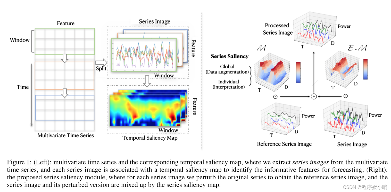
Figure 1: (Left): multivariate time series and the corresponding temporal saliency map, where we extract series images from the multivariate time series, and each series image is associated with a temporal saliency map to identify the informative features for forecasting; (Right): the proposed series saliency module, where for each series image we perturb the original series to obtain the reference series image, and the series image and its perturbed version are mixed up by the series saliency map.

图1:(左):多元时间序列和相应的时间显著图，我们从多元时间序列中提取序列图像，每个序列图像与一个时间显著图相关联，以识别用于预测的信息特征;(右):提出的序列显著性模块，对每个序列图像扰动原序列得到参考序列图像，序列图像与其扰动后的版本通过序列显著性图进行混合。

2 Methods

We now present our method in detail, which consists of a series saliency module and its use in both training and interpretation phases.

我们现在详细介绍了我们的方法，它包括一系列显著性模块及其在训练和解释阶段的使用。

2.1 Setup and Notations

As shown in Fig. 1, multivariate time series data are spatiotemporal with two dimensions – time and feature. Formally, we use S to denote a series of observed time series signal:
$S=[s1,s2,\cdot \cdot \cdot ,st,\cdot \cdot \cdot ],(1)$

where $s_t\in R^D$ denotes the feature vector with dimension $D$ at time $t$. For every time step $t$, we aim to predict the future value $s_{t+\tau }$after a given horizon $\tau$. The horizon is chosen according to the forecasting task settings. For example, for the traffic usage, the horizon τ of interest ranges from an hour to a day; while for the stock market data, even a second or minute ahead forecasting can be meaningful for generating returns. Besides forecasting accuracy, we are also interested in interpretation: which features contribute most and which contributes least for the final forecast predictions? As stated above, traditional statistical methods (e.g., [Box and Jenkins, 1976] and [Harvey, 1990]) are easy to interpret by making some explicit model assumptions that can extract interpretations directly from the learned model parameters, while they are often limited in forecasting accuracy.

In contrast, recent progress on deep learning methods leads to superior prediction capabilities [Goodfellow et al, 2016], however, they are hard to interpret since the deep model assumptions are stacked with multiple non-linear activation or blocks.
A key part of an effective model for multivariate time series forecasting would be the capability on handling the information from both time and feature dimensions in a coherent manner. Recent work develops an attention-basedscheme [Assaf et al, 2019; Shih et al, 2019], which introduces an attention map to “selectively” combine time-feature information (see Fig. 2 (left)), with the primary focus on interpretation. However, as pointed out in [Ismail et al, 2020], the attention-based methods can be insufficient for interpreting multivariate time-series data. We develop a new scheme of series saliency, which is model-agnostic and can boost both forecasting accuracy and interpretation, as detailed below.

如图1所示，多元时间序列数据具有时间和特征两个维度的时空特征。形式上，我们用S表示一系列观测到的时间序列信号:

$$S=[s_1,s_2,\cdot \cdot \cdot ,s_t,\cdot \cdot \cdot ],\text{\hspace{1em}(1)}$$

其中$s_t\in R^D$表示时间t时维度为$D$的特征向量。对于每个时间步$t$，我们的目标是预测给定视界$\tau$后的未来值$s_{t+\tau }$。根据预测任务设置选择视界。例如，对于流量使用情况，感兴趣的地平线$\tau$范围从一小时到一天;而对于股市数据，即使是提前一秒钟或一分钟的预测，对产生回报也是有意义的。除了预测的准确性，我们还对解释感兴趣:哪些特征对最终的预测贡献最大，哪些贡献最小?如上所述，传统的统计方法(如[Box and Jenkins, 1976]和[Harvey, 1990])很容易通过做出一些明确的模型假设来解释，这些假设可以直接从学习到的模型参数中提取解释，但它们往往在预测精度方面受到限制。

相比之下，深度学习方法的最新进展导致了卓越的预测能力[Goodfellow等人，2016]，然而，它们很难解释，因为深度模型假设堆叠了多个非线性激活或块。

有效的多元时间序列预测模型的一个关键部分是以连贯的方式处理来自时间和特征维度的信息的能力。最近的工作开发了一种基于注意力的计划[Assaf等人，2019;Shih等人，2019]，他们引入了一种注意力图，以“选择性地”结合时间特征信息(见图2(左))，主要关注解释。然而，正如[Ismail等人，2020]所指出的那样，基于注意力的方法可能不足以解释多元时间序列数据。我们开发了一种新的序列显著性方案，它是模型不可知的，可以提高预测精度和解释，如下所述。

2.2 Series Saliency

We develop series saliency by drawing inspirations from the saliency maps [Dabkowski and Gal, 2017] in computer vision. However, unlike previous work on saliency maps that mainly focuses on interpetability of deep models, series saliency is beneficial for improving both forecasting accurarcy and interpretation for time-series data.

Specifically, to consider the time-feature information jointly, we first represent the multivariate time series as a set of 2D series images. As shown in Fig. 1, each series image corresponds to a part of the multivariate time series within a given time window. Formally, let $T$ be the window size. We simply set the value of $T$ for various datasets with 2 periodic patterns (e.g., $p=48$ for hourly electricity consumption). A series image is represented as a matrix $X\in R^{D\times T}$ , of which each row corresponds to one feature dimension in the multivariate time series. Then, we follow the perturbation strategy in the smallest destroying region (SDR) principle [Dabkowski and Gal, 2017] to design the series saliency scheme. We define a reference series image $X$ by adding noise or Gaussian blur on each element of the original series image $X$:
$${\hat{x}}_{t,i}=\{\begin{array}{l}{x}_{t,i}+{ϵ}_{{\sigma }_1},noise\\ g_{{\sigma }_2}(x_{t,i}),blur\end{array}\text{\hspace{1em}(2)}$$
where ${ϵ}_{{\sigma }_1}\sim \mathcal{N}\left(\mu ,{\sigma }_1^2\right)$is a Gaussian noise and $\sigma 2$ is a Gaussian blur kernel on element xt,i with the maximum isotropic standard deviation $\sigma 2$

我们通过从计算机视觉中的显著图[Dabkowski和Gal, 2017]中汲取灵感来开发系列显著性。然而，与以往对显著性图的研究主要关注深度模型的互操作性不同，序列显著性有利于提高时间序列数据的预测精度和解释。

具体来说，为了综合考虑时间特征信息，我们首先将多元时间序列表示为一组二维序列图像。如图1所示，在给定的时间窗口内，每个序列图像都对应于多元时间序列的一部分。形式上，设$T$为窗口大小。我们简单地为具有2个周期模式的各种数据集设置$T$的值(例如，每小时用电量的$p=48$)。序列图像表示为矩阵$X\in R^{D\times T}$，其中每一行对应多元时间序列中的一个特征维。然后，我们遵循最小破坏区(SDR)原理的扰动策略[Dabkowski and Gal, 2017]设计了序列显著性方案。我们通过在原始系列图像$X$的每个元素上添加噪声或高斯模糊来定义参考系列图像$X$:

$${\hat{x}}_{t,i}=\{\begin{array}{l}{x}_{t,i}+{ϵ}_{{\sigma }_1},noise\\ g_{{\sigma }_2}(x_{t,i}),blur\end{array}\text{\hspace{1em}(2)}$$

${ϵ}_{{\sigma }_1}\sim \mathcal{N}\left(\mu ,{\sigma }_1^2\right)$是一个高斯噪声，$g_{{\sigma }_2}$是元素$x_{t,i}$上的一个高斯模糊核blur kernel，其各向同性标准差最大${\sigma }_2$

In time series data, each series can be composed of three parts — trend, seasonality and residual [Hyndman and Athanasopoulos, 2018]. As shown in [Hyndman and Athanasopoulos, 2018], blurring is helpful to extract the trend information of a time series, and adding some noise can enhance the local information. When the amount of injected noise or blurring is small, the reference series images can be treated as data augmentation in the time domain [Iwana and Uchida, 2020] to learn deep models. However, if the noise (or blurring) is not set properly (e.g., too large), the noise (or blurring) will introduce irregular roughness to cover the original series, making it difficult for DNNs to learn temporal patterns in reference data.

在时间序列数据中，每个序列可以由趋势、季节性和残差三部分组成[Hyndman and Athanasopoulos, 2018]。如[Hyndman and Athanasopoulos, 2018]所示，blurring有助于提取时间序列的趋势信息，添加一些噪声可以增强局部信息。当注入noise 或blurring很小时，可以将参考系列图像视为时域数据增强[Iwana and Uchida, 2020]来学习深度模型。然而，如果噪声(或模糊)设置不当(例如过大)，噪声(或模糊)将引入不规则的粗糙度来覆盖原始序列，使dnn难以学习参考数据中的时间模式。

To relieve the sensitivity over noise (or blurring), the series saliency module further introduces a learnable mask $M\in [0,1{]}^{D\times T}$ and selectively combines the reference series image and the original one:
$$\tilde{X}=M\odot \hat{X}+\left(E-M\right)\odot X\text{\hspace{1em}(3)}$$where E is the matrix with all elements be the unit one. As illustrated in Fig. 1, in such a design, the series saliency module can generate data (i.e., $\tilde{X}$) that cover the unexplored input space while maintaining the important characteristics of the original series image (i.e., $X$). As we shall see, series saliency is an effective data augmentation strategy for training deep models and it is learnable.

Besides augmenting the data for improving training, series saliency can also be used for interpretation by simply changing the objective to be optimized. We defer the details to Section 2.4 after presenting the training procedure.

为了缓解对噪声(或模糊blurring)的敏感性，序列显著性模块进一步引入了一个可学习的掩码
$M\in [0,1{]}^{D\times T}$，并有选择地将参考序列图像与原始图像相结合:
$$\tilde{X}=M\odot \hat{X}+\left(E-M\right)\odot X\text{\hspace{1em}(3)}$$

其中$E$是矩阵，所有元素都是单位1。如图1所示，在这样的设计中，序列显著性模块可以生成覆盖未探索的输入空间的数据(即$\tilde{X}$)，同时保持原始序列图像(即$X$)的重要特征。我们可以看到，序列显著性是训练深度模型的一种有效的数据增强策略，并且是可学习的。

除了增加数据以改进训练外，序列显著性还可以通过简单地改变要优化的目标来用于解释。在介绍了培训程序之后，我们将细节推迟到第2.4节。

2.3 Training with Series Saliency

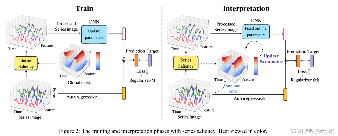
With the series saliency module, we now present the entire model architecture and its training details. One essential problem in deep learning models is that the scale of the outputs is not sensitive to the scale of inputs. In specific real time series datasets, the scale of input data often changes in a non-periodic manner, which can significantly lower the fore casting accuracy of deep learning models. We propose to decompose the final prediction into a linear part, which primarily focuses on the local scaling issue, plus a non-linear part containing complex temporal patterns. Fig. 2 (left) shows the dual-path architecture — a nonlinear deep learning (DL) module and a linear auto-regressive (AR) module.

The original series images $X$ are converted to the processed versions $\tilde{X}$ by our proposed module, and then $\tilde{X}$ are fed into the DL module to obtain $y^{(r)}$. Here, the DL module can be any time series network, e.g., convolution neural networks, recurrent neural networks, Long short-term memory (LSTM) [Hochreiter and Schmidhuber, 1997], long- and short-term temporal pattern neural network (LSTNet) [Lai et al, 2018] and Self-Attention encoder [V aswani et al, 2017] (see experiments for details). For the linear part, we choose an auto-regressive model and denote its result as $y^{(o)}$:
$$y^{\left(o\right)}=\sum _{k=0}^p{W}_k^{\top }{y}_{t-k}+b,\text{\hspace{1em}(4)}$$
where $p$ is the order of the AR model, $W_k\in R^D$ and $b\in R$ are its coefficients. p can be determined for various datasets with periodic patterns (e.g., $p=24$ for the hourly electricity consumption). In our experiments, we empirically searched a good p through validation. The final forecasting is obtained by combining the outputs of both DL and AR:
$$\hat{y}=y^{\left(o\right)}+y^{\left(r\right)}.\text{\hspace{1em}(5)}$$
Let $N$ be the number of series images in the training set and Φ = { θ , W , b } Φ =\{θ, W, b\} Φ={ θ,W,b} denote all the unknown parameters. For notation simplicity, we will use $y_i$ to denote the ground-truth forecasting result of $X_i$ at a particular horizon. We adopt stochastic gradient descent (SGD) to jointly optimize over $\Phi$ and $M$. Specifically, at each iteration, we draw a mini-batch $B=(Xi,yi)ni=1$with size n. Our loss function ‘$(\Phi ,M)$ consists of two parts. First, for each $(Xi,yi)$ ∈ B, we follow the diagram in Fig. 2 to get the prediction ${\hat{y}}_i$(a function of both $\phi$ and $M$) via Eq. (5), and accumulate the squared error $\Vert {\hat{y}}_i-y_i{\Vert }^2$ into the loss $l(\Phi ，M)$. Second, to fully leverage the training set, we also send the original series image Xi into both the DNN and AR model (i.e., bypassing the series saliency module in Fig. 2 to get another prediction ˆy0i (a function of φ only) via Eq. (5), and accumulate the squared error kˆy0i − yik2 into the loss ‘(φ, M). Our overall training objective is to minimize a regularized version of loss$l(\Phi ，M)$:
$${\mathcal{L}}_1\left(\Phi ,M\right)=l\left(\Phi ,M\right)+{\lambda }_1{l}_m\left(M\right)+{\lambda }_2{l}_r\left(M\right),\text{\hspace{1em}(6)}$$
where $l_m\left(M\right)$and$l_r\left(M\right)$are regularization terms on the mask $M$, $\lambda 1$ and$\lambda 2$ are the corresponding coefficients.
The effect of the regularizer$l_m\left(M\right)$is to control the amount of perturbation. As stated before, if $M$ is close to $E$, the reference series image will dominate and may degenerate the performance. To discourage such degenerating case, we choose the common 2-norm, i.e., $l_m\left(M\right)=\Vert M{\Vert }^2$.
The design of ‘r(M) is a bit more subtle. Note that a key difference exists between our series images and the natural images in computer vision — the rows (i.e., features) of series images are permutable without affecting the content, while switching the rows of a nature image would destroy its semantic meaning. In our case, we would expect the feature importance matrix M to be row-wisely orthogonal. Therefore, we define the regularizer term
$$l_r\left(M\right)=\Vert {M{M}^{\top }-I\Vert }_F,\text{\hspace{1em}(7)}$$
where $I$ is the identity matrix and$\Vert {\cdot \Vert }_F$is the Frobenius norm.
Such orthogonality is beneficial for interpretation, and can boost the training as well (see ablation study in Section 3.2).
With the overall objective L1, we use back-propagation to calculate its gradient and apply SGD to update$(\Phi ，M)$. We would like to highlight a key difference from the traditional data augmentation [Iwana and Uchida, 2020]. Unlike the traditional methods, which typically augment the data for once with some pre-fixed strategies (e.g., perturbation with a fixed noise), our augmentation strategy is adaptive by iteratively updating the mask $M$ of the series saliency module. Such a scheme makes the model to better focus on informative parts that are good for forecasting, as we shall see in experiments.

使用Series Saliency模块，我们现在展示整个模型架构及其训练细节。深度学习模型的一个基本问题是输出的规模对输入的规模不敏感。在特定的实时序列数据集中，输入数据的尺度往往会发生非周期性的变化，这会显著降低深度学习模型的预测精度。我们建议将最终预测分解为主要关注局部尺度问题的线性部分，以及包含复杂时间模式的非线性部分。图2(左)显示了双路径架构——一个非线性深度学习(DL)模块和一个线性自回归(AR)模块。

我们提出的模块将原始系列图像X转换为处理后的版本 $\tilde{X}$，然后将 $\tilde{X}$输入DL模块得到$y^{(r)}$。在这里，DL模块可以是任何时间序列网络，例如卷积神经网络、循环神经网络、长短期记忆(LSTM) [Hochreiter和Schmidhuber, 1997]、长短期时间模式神经网络(LSTNet) [Lai等人，2018] 和自注意编码器[ V aswani等人，2017] (详情见实验)。对于线性部分，我们选择一个自回归模型，并将其结果表示为$y^{(o)}$:
$$y^{\left(o\right)}=\sum _{k=0}^p{W}_k^{\top }{y}_{t-k}+b,\text{\hspace{1em}(4)}$$
其中p是AR模型的阶数， $W_k\in R^D$ 和$b\in R$是它的系数。对于具有周期性模式的各种数据集，可以确定$p$(例如，每小时耗电量的$p=24$)。在我们的实验中，我们通过验证经验地搜索了一个好的$p$。结合DL和AR的输出得到最终的预测结果:
$$\hat{y}=y^{\left(o\right)}+y^{\left(r\right)}.\text{\hspace{1em}(5)}$$

设N为训练集中序列图像的个数， Φ = { θ , W , b } Φ =\{θ, W, b\} Φ={ θ,W,b}表示所有未知参数。为了简化符号，我们将使用yi表示$X_i$在特定时间段的实际预测结果。我们采用随机梯度下降法$(SGD)$对$\Phi$和$M$进行联合优化。具体来说，在每次迭代中，我们都会得到一个大小为$n$的mini-bactch B = { ( X i , y i ) } i = 1 n B=\left\{ \left( X_i,y_i \right) \right\} _{i=1}^{n} B={ (Xi​,yi​)}i=1n​。我们的损失函数$l(\Phi ，M)$由两部分组成。首先，对于每个$(X_i,y_i)$∈B，我们按照图2中的图通过公式（5）得到预测值ˆyi（$\Phi$和$M$的函数），并将平方误差$\Vert {\hat{y}}_i-y_i{\Vert }^2$累加到损失$l(\Phi ，M)$中。其次，为了充分利用训练集，我们还将原始序列图像$X_i$发送到DNN和AR模型中（即绕过图2中的序列显著性模块，通过等式（5）得到另一个预测${\hat{y}}_i^{\prime }$（仅为$\Phi$的函数），并将平方误差$\Vert {\hat{y}}_i^{\prime }-y_i{\Vert }^2$累加到损失$l(\Phi ，M)$中。我们的总体培训目标是尽量减少损失的正规化版本$l(\Phi ，M)$：

$${\mathcal{L}}_1\left(\Phi ,M\right)=l\left(\Phi ,M\right)+{\lambda }_1{l}_m\left(M\right)+{\lambda }_2{l}_r\left(M\right),\text{\hspace{1em}(6)}$$

其中$l_m\left(M\right)$和$l_r\left(M\right)$为掩模$M$上的正则化项，${\lambda }_1$和${\lambda }_2$为对应系数。

正则子$l_m\left(M\right)$的作用是控制扰动量。如前所述，如果$M$接近$E$，则参考序列图像将占主导地位，可能会使性能下降。为了防止这种退化情况，我们选择了公共2范数，即$l_m\left(M\right)=\Vert M{\Vert }^2$。

$l_m\left(M\right)$的设计更微妙一些。请注意，在计算机视觉中，我们的系列图像和自然图像之间存在一个关键的区别——系列图像的行(即特征)是可替换的，而不会影响内容，而切换自然图像的行将破坏其语义。在我们的例子中，我们期望特征重要性矩阵$M$是行明智正交的。因此，我们定义正则项$l_m\left(M\right)$:
$$l_r\left(M\right)=\Vert {M{M}^{\top }-I\Vert }_F,\text{\hspace{1em}(7)}$$

其中$I$是单位矩阵，$\Vert {\cdot \Vert }_F$是Frobenius范数。这种正交性有利于解释，也可以促进训练(见3.2节的消融研究)。
对于总体目标${\mathcal{L}}_1$，我们使用反向传播来计算其梯度，并应用$SGD$来更新$(\Phi ，M)$。我们想强调与传统数据增强的一个关键区别[Iwana和Uchida, 2020]。与传统方法不同，传统方法通常使用一些预先固定的策略(例如，用固定噪声扰动)对数据进行一次增强，我们的增强策略是通过迭代更新序列显著性模块的掩码$M$来自适应的。正如我们将在实验中看到的那样，这样的方案使模型更好地关注于有利于预测的信息部分。

2.4 Interpretation with Series Saliency

Now, we show that with the series saliency module, we can easily derive an interpretation strategy for forecasting.
Let $X^{\ast }$ be the a series image in the testing set with groundtruth forecasting y∗ at a particular horizon$\tau$. Let${\Phi }^{\ast }$ denote the optimal parameters of the DNN and AR models after training. We follow the diagram in Fig. 2 to get the prediction $y^{\ast }$ (a function of $M$) via Eq. (5), and calculate the squared error$\Vert {\hat{y}}^{\ast }-y^{\ast }{\Vert }^2$. The goal of interpretation is to find the most salient evidence that influences the model performance measured by square error. In series saliency, the most salient feature regions are found by identifying the highly representative mask, which summarizes compactly the effect of deleting feature regions, either setting values to zeros or Gaussian noise, to explain the behaviour of the DL part. For the AR part, the weights are easy-to-interpret because of its linearity [Hyndman and Athanasopoulos, 2018]. On the other hand, the AR part mainly assists DL models to address the local scaling issue, so it is not essential to focus on the explanation of the AR part. Formally, we formulate interpretation as minimizing the following objective:
$$L_2\left(M;X^{\ast }\right)=-\Vert {\hat{y}}^{\ast }-y^{\ast }{\Vert }^2+{\lambda }_1{l}_m\left(M\right)+{\lambda }_2{l}_r\left(M\right),\text{\hspace{1em}(8)}$$
where $l_m\left(M\right)$and$l_r\left(M\right)$are the same regularization terms as in training. Then, we use back-propagation to calculate the gradient of L2 and apply SGD to update M only. After convergence, the optimal M provides an interpretation of important features for forecasting on instance$X^{\ast }$.

现在，我们展示了使用序列显著性模块，我们可以很容易地推导出预测的解释策略。

设$X^{\ast }$为在特定视界$\tau$处具有真实值预测$y^{\ast }$的测试集中的a序列图像。设${\Phi }^{\ast }$表示训练后DNN和AR模型的最优参数。我们根据图2中的图表，通过Eq.(5)得到预测函数$y^{\ast }$ ($M$的函数)，并计算平方误差$\Vert {\hat{y}}^{\ast }-y^{\ast }{\Vert }^2$。解释的目标是找到影响由平方误差测量的模型性能的最显著的证据。在序列显著性中，通过识别具有高度代表性的掩码来发现最显著的特征区域，它紧凑地总结了删除特征区域的效果，将值设置为零或高斯噪声，以解释DL部分的行为。对于AR部分，由于其线性性，权重易于解释[Hyndman和Athanasopoulos, 2018]。另一方面，AR部分主要是帮助DL模型解决局部缩放问题，因此不必关注AR部分的解释。形式上，我们将解释定义为最小化以下目标:
$$L_2\left(M;X^{\ast }\right)=-\Vert {\hat{y}}^{\ast }-y^{\ast }{\Vert }^2+{\lambda }_1{l}_m\left(M\right)+{\lambda }_2{l}_r\left(M\right),\text{\hspace{1em}(8)}$$

其中$l_m\left(M\right)$和$l_r\left(M\right)$是训练中相同的正则化项。然后，我们使用反向传播计算$L_2$的梯度，并应用$SGD$仅更新$M$。收敛后，最优$M$为实例$X^{\ast }$的预测提供了重要特征的解释。

3 Experiments

We now present experimental results by comparing the performance of four widely-used deep learning models with and without the proposed series saliency module on various datasets. We also give an ablation study on the mask and AR model components. Then we show extensive qualitative results on how saliency heatmaps interpret the forecasts.

现在，我们通过比较四种广泛使用的深度学习模型在不同数据集上的性能，并将其与未提出的序列显著性模块进行比较。我们还对掩模和AR模型组件进行了烧蚀研究。然后，我们展示了显著性热图如何解释预测的广泛定性结果。

3.1 Experimental Setting

(1) Datasets: We use three time series datasets electricity, Air-quality, Industry data The three datasets are representative (from difficult to easy).
(2) Metrics: We use two evaluation metrics, namely relative squared error (RSE) and empirical correlation coefficient (CORR). For RSE, lower values are better, while for CORR higher values are better. The datasets and the metrics have been widely used in many papers about time series forecasting (e.g., LSTNet, TPA-LSTM) [Lai et al, 2018; Shih et al, 2019].
(3) Deep Learning Module: We use four state-of-the-art architectures for comparison (i.e., CNN, GRU+Attention, LSTNet and Self-Attention encoder).
These four deep learning models achieve superior forecasting performance and in the following results they are used as the deep learning module to get interpreted by the proposed series saliency method.

(1)数据集: 我们使用三个时间序列数据集电力、空气质量、工业数据。这三个数据集具有代表性(从难到易)。
(2)指标: 我们使用了两个评价指标，即相对平方误差(RSE)和经验相关系数(CORR)。RSE值越低越好，CORR值越高越好。数据集和指标已广泛用于许多关于时间序列预测的论文(例如，LSTNet, TPA-LSTM) [Lai等人，2018;Shih等，2019]。
(3)深度学习模块: 我们使用四种最先进的架构进行比较(即CNN, GRU+Attention, LSTNet和Self-Attention encoder)。

这四个深度学习模型都取得了优异的预测性能，在下面的结果中，它们被用作深度学习模块，并用所提出的序列显著性方法进行解释。

3.2 Results on Forecasting

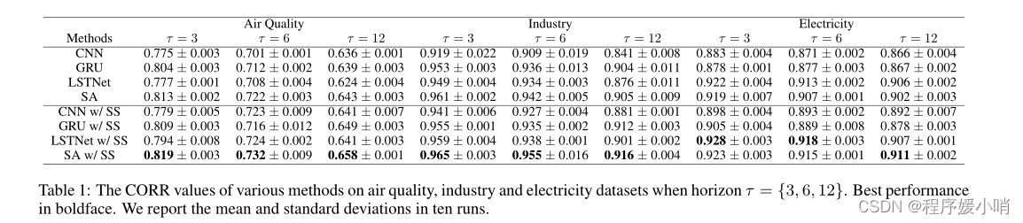
Table 1 presents the CORR values of various methods on the three datasets with different forecasting horizons. We can see that using the series saliency module can boost the forecasting accuracy of various deep models on the Air quality dataset, especially when the forecasting horizon is large. This is because the model complexity increases with the horizon, and data augmentation may help explore more useful temporal information. We also observe that among all the deep architectures in comparison, the Self-Attention encoder with the series saliency gives the best performance in most settings, mainly because of the powerful representation capability of the transformer encoder model. Therefore, in the sequel, we will use the Self-Attention encoder as the main architecture to do further analysis.

表1给出了不同预测层数的三个数据集上各种方法的CORR值。我们可以看到，使用序列显著性模块可以提高各种深度模型在空气质量数据集上的预测精度，特别是在预测视界较大时。这是因为模型的复杂性随着视界的增加而增加，而数据增强可能有助于探索更多有用的时间信息。我们还观察到，在比较的所有深度架构中，具有系列显著性的Self-Attention编码器在大多数情况下表现最好，这主要是因为变压器编码器模型具有强大的表示能力。因此，在后续中，我们将以Self-Attention编码器作为主要架构来做进一步的分析。

Ablation Study

We now present an ablation study to demonstrate the effectiveness of our design components, including regularization terms and and the auto-regressive path in our architecture.
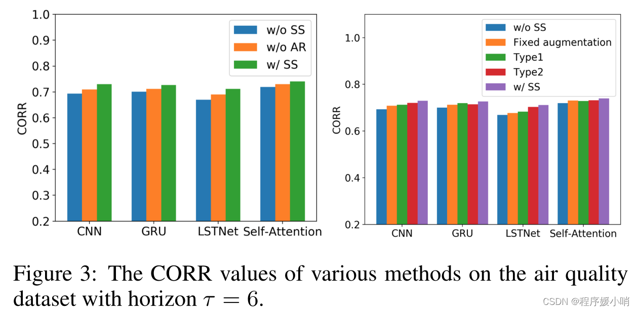
First, we examine how the auto-regressive module helps on the forecasting when series saliency (i.e., data augmentation) is used. We compare the following variants:

• w/ SS: The model in Fig. 2 with series saliency (SS).
• w/o SS: The model in Fig. 2, but without series saliency;
• w/o AR: The model in Fig. 2 with series saliency, but without the auto-regressive component.

Fig. 3 (left) shows the results. We do not use any perturbation in w/o SS. We can see that both the series saliency (i.e., adaptive data augmentation) and the auto-regressive modules are helpful to boost the performance — dropping either one would lead to degenerated performance.
Second, we do a finer investigation on the effects of the regularization terms in learning the series saliency module during training. We compare the following variants:

• w/o SS: The model in Fig. 2, but without the series saliency module (i.e., no data augmentation);

• Fixed augmentation: Augment the series images for once with some prefixed strategies (perturbation with a fixed noise) [Iwana and
  Uchida, 2020].

• Type1: The entire model in Fig. 2 trained by minimizing the loss only (i.e., without ‘r and ‘m).

• Type2: The entire model in Fig. 2 trained by minimizing the loss with ‘m regularizer (i.e., without ‘r).

• w/ SS: The entire model in Fig. 2 trained with both ‘r and ‘m regularizers as in Eq. (6).

Fig. 3 (right) shows the results. Again, we can see that series saliency can boost the forecasting results (i.e., higher CORR). Also, being an adaptive strategy, series saliency is more effective for training deep models than the pre-fixed data augmentation method [Iwana and Uchida, 2020]. The regularizer term ‘m has little effect on improving the model performance, while ‘r is much more influential. By considering the decouple of feature importance in time series help the neural networks understand time series data accurately.

我们现在提出一个消融研究，以证明我们的设计组件的有效性，包括正则化术语和自回归路径在我们的架构。

首先，我们研究了在使用序列显著性(即数据增强)时，自回归模块如何帮助预测。我们比较以下变体:

• w/ SS:图2中具有序列显著性(SS)的模型。
• w/o SS:模型如图2所示，但无序列显著性;
• w/o AR:图2中具有序列显著性的模型，但不含自回归分量。

结果如图3(左)所示。我们没有在w/o SS中使用任何扰动。我们可以看到，序列显著性(即自适应数据增强)和自回归模块都有助于提高性能——降低其中任何一个都会导致性能退化。

其次，我们更细致地研究了正则化项在训练过程中学习序列显著性模块时的影响。我们比较以下变体:

• w/o SS:图2中的模型，但没有序列显著性模块(即没有数据增强);•固定增强:使用一些前缀策略(固定噪声扰动)对系列图像进行一次增强[Iwana和Uchida, 2020]。

• Type1:图2中的整个模型仅通过最小化损失进行训练(即不包含’ r ‘和’ m)。

• Type2:图2中的整个模型通过使用’ m正则子最小化损失来训练(即不使用’ r)。

• w/ SS:图2中的整个模型使用公式(6)中的’ r ‘和’ m正则子进行训练。

结果如图3(右)所示。同样，我们可以看到序列显著性可以提高预测结果(即更高的CORR)。此外，作为一种自适应策略，序列显著性在训练深度模型时比预先固定的数据增强方法更有效[Iwana和Uchida, 2020]。正则项’ m对提高模型性能影响不大，而’ r的影响要大得多。考虑特征重要性在时间序列中的解耦，有助于神经网络对时间序列数据的准确理解。

3.3 Results on Interpretation

We present both qualitative and quantitative results.

我们给出了定性和定量结果。

Qualitative Analysis

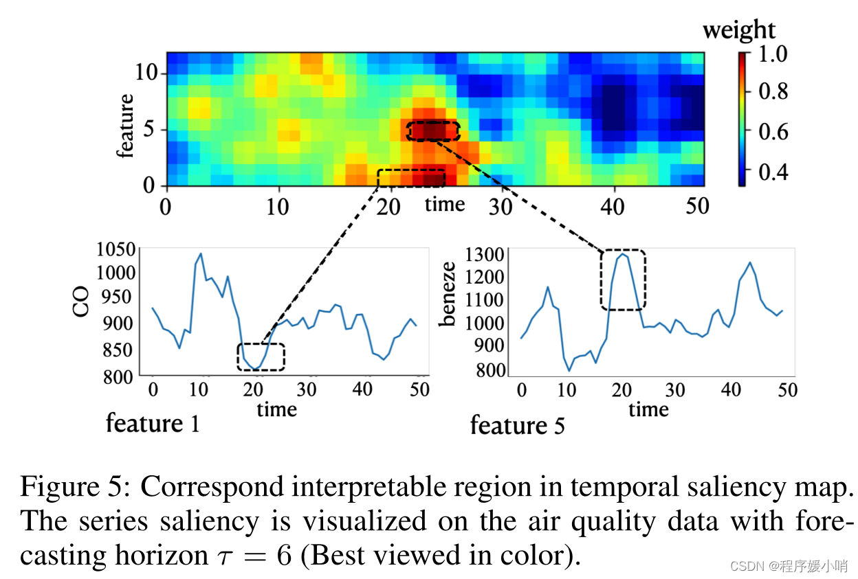
We apply the series saliency methods with the Self-Attention encoder model on the air quality dataset. Fig. 5 visualizes the learned mask component when forecasting the selected future value with horizon τ = 6. As the color bar shows, from blue to red means that the features become more and more important. We can see that the features from time interval [20, 30] have the largest saliency, which corresponds to the extremelow value in feature 1 representing the concentration of CO and high value in feature 5 representing the concentration of benzene.

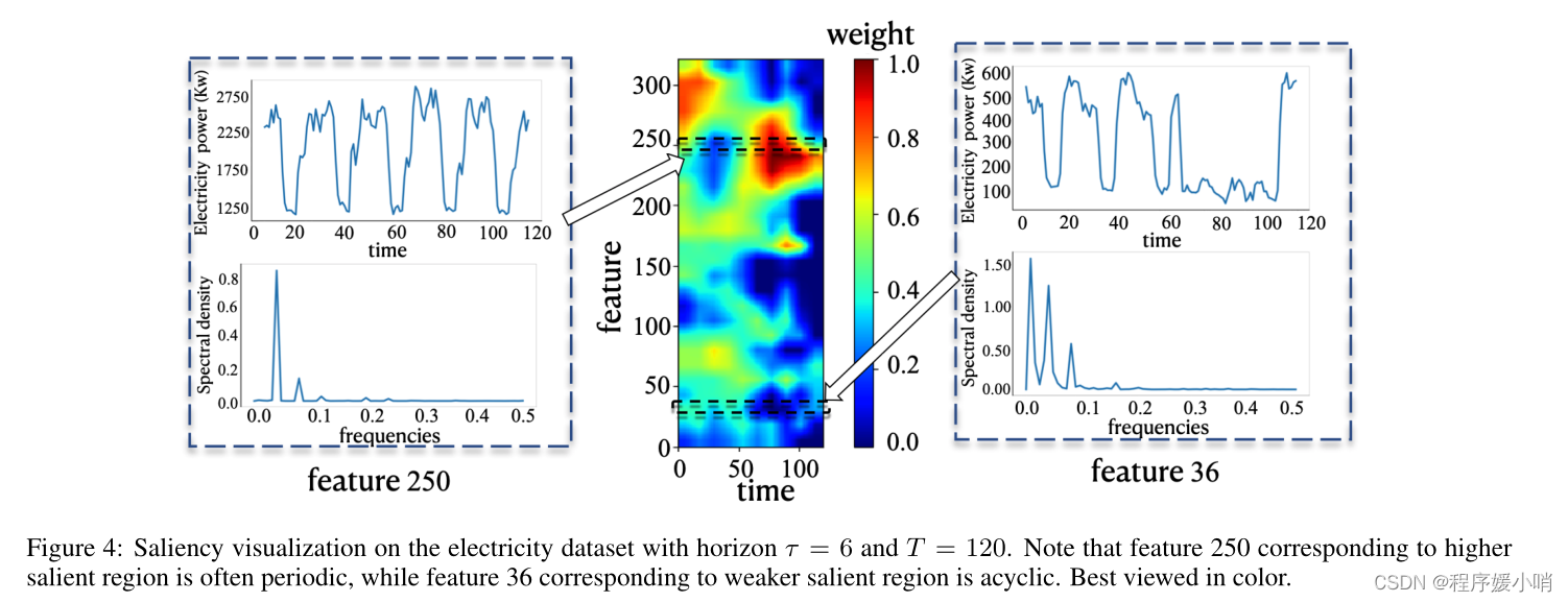
We also visualize the correspondence between saliency mask, the original time series data and the data frequencies on the electricity dataset. Fig. 4 shows the results. We can see that the data of channel 250 has the high value of the saliency mask and reflects a periodic structure (top left in Fig. 4). In contrast, the data of channel 36 has the low value of the saliency mask and reflects a relatively acylic structure (top right in Fig. 4). Furthermore, to prove the periodicity of our selected a channels, we map the corresponding feature to a frequency domain by a fast fourier transform procedure (FFT) [Nussbaumer, 1981] and show the frequency result below the data of the two channels.

我们将序列显著性方法和自注意编码器模型应用于空气质量数据集。图5显示了当水平$\tau =6$时预测所选未来值时学习到的掩模分量。正如颜色条所示，从蓝色到红色意味着特征变得越来越重要。我们可以看到，时间段[20,30]的特征显著性最大，对应于特征1中代表CO浓度的极值和特征5中代表苯浓度的高值。

我们还可视化了显著性掩码、原始时间序列数据和电力数据集上的数据频率之间的对应关系。结果如图4所示。我们可以看到，250通道的数据显著掩码值较高，反映了一个周期结构(图4左上)。相反，36通道的数据显著掩码值较低，反映了一个相对无环的结构(图4右上)。此外，为了证明我们所选通道的周期性，我们通过快速傅里叶变换程序(FFT)将相应的特征映射到频域[Nussbaumer，1981]，并在两个频道的数据下面显示频率结果。

Quantitative Comparison

Finally, similar as in [Ismail et al, 2020], we present a quantitative metric to evaluate the interpretability for time series forecasting and compare with various baselines.

Specifically, for each testing example X, we use a given interpretation method to generate the feature importance map, and select the top k features. Then, we add the random Gaussian noise on the selected features, and feed the perturbed version into the pretrained model for forecasting. Given a testing set, we calculate the corresponding CORR value. We change the value of k = [10%, …, 90%], and obtain the decreasing CORR curve with different k (i.e., different perturbation levels). Finally, we calculate the area under the CORR curve as the quantitative metric and denote it by AUCORR. The lower AUCORR values mean that we select the more important features ßand the interpretation method is more effective.

We compare with a wide range of baselines including Grad [Baehrens et al, 2010], DeepLift [Shrikumar et al, 2017], feature ablation [Suresh et al, 2017], Occlu-sion [Zeiler and Fergus, 2014], Shapely sampling [Castro et al, 2009] and attention [Petersen and Posner, 2012]. Also, to examine the effect of regularizers in interpretation, we consider the following variants of our method:

• w/ SS: The model in Fig. 2 interpreted with both ‘r and ‘m regularizers as in Eq. (8);
• Type1: The model in Fig. 2 interpreted by minimizing the loss L2 only (i.e., without ‘r and ‘m);
• Type2: The model in Fig. 2 interpreted by minimizing the loss L2 with ‘r regularizer (i.e., without ‘m).

Table 2 and Fig. 6 show the results. We can see that the series saliency map by our method can obtain the best quantitative interpretation results compared to those by other interpretation results (e.g., DeepLift and attention). Moreover, the two regularization terms $l_m\left(M\right)$和$l_r\left(M\right)$ are useful to improve the interpretation results. In general, although we can’t guarantee any selected future values will have the representative interpretation in qualitative analysis (e.g., Fig. 5), the performance of our method is quantitatively superior to other competitors.

最后，与[Ismail等人，2020]类似，我们提出了一个定量度量来评估时间序列预测的可解释性，并与各种基线进行比较。

具体来说，对于每个测试示例X，我们使用给定的解释方法生成特征重要性图，并选择前k个特征。然后，在选定的特征上添加随机高斯噪声，并将扰动后的特征输入预训练模型进行预测。给定一个测试集，我们计算相应的CORR值。我们改变k =[10%，…]， 90%]，得到不同k(即不同摄动水平)下的CORR递减曲线。最后，我们计算CORR曲线下的面积作为定量度量，并用AUCORR表示。AUCORR值越低，说明我们选择了更重要的特征ß，解释方法越有效。

我们比较了广泛的基线，包括Grad [Baehrens等人，2010年]，DeepLift [Shrikumar等人，2017年]，特征消融[Suresh等人，2017年]，occlusion [Zeiler和Fergus, 2014年]，Shapely采样[Castro等人，2009年]和注意力[peterson和波斯纳，2012年]。此外，为了检查正则子在解释中的影响，我们考虑了我们方法的以下变体:

• w/ SS:图2中的模型如Eq.(8)所示，使用’ r ‘和’ m正则子解释;
• Type1:图2中的模型仅通过最小化损失L2来解释(即，不包含$l_m\left(M\right)$和$l_r\left(M\right)$;
• Type2:图2中的模型，用’ r正则子最小化损失$L_2$(即不带$m$)来解释。

结果如表2和图6所示。我们可以看到，与其他解释结果(如DeepLift和attention)相比，我们的方法得到的序列显著图可以获得最好的定量解释结果。此外，两个正则化项$l_m\left(M\right)$和$l_r\left(M\right)$有助于改善解释结果。总的来说，虽然我们不能保证任何选择的未来值在定性分析中具有代表性的解释(如图5)，但我们的方法在定量上优于其他竞争者。

4 Conclusions

We present a novel scheme of series saliency to boost both accuracy and interpretability for multivariate time series forecasting. By extracting series images from sliding windows of the time series, we design series saliency as a mixup approach with a learnable mask defined on the series images and their perturbed versions. Series saliency acts as an adaptive data augmentation method for training deep models, and meanwhile by slightly changing the objective, it can be optimized to find a mask for interpretable forecasting in both feature and time dimensions. Experimental results show the superiority of series saliency over various baselines.

我们提出了一种新的序列显著性方案，以提高多元时间序列预测的准确性和可解释性。通过从时间序列的滑动窗口中提取序列图像，我们将序列显著性设计为一种混合方法，并在序列图像及其扰动版本上定义了可学习掩码。序列显著性是一种自适应的数据增强方法，用于训练深度模型，同时通过稍微改变目标，可以在特征和时间维度上优化找到一个可解释预测的掩码。实验结果表明，序列显著性优于各种基线。