像长期短期记忆(LSTM)神经网络的神经网络能够模拟多个输入变量的问题。这在时间序列预测中是一个很大的益处,其中古典线性方法难以适应多变量或多输入预测问题。
在本教程中,您将发现如何在Keras深度学习库中开发多变量时间序列预测的LSTM模型。
完成本教程后,您将知道:
- 如何将原始数据集转换为可用于时间序列预测的内容。
- 如何准备数据并适应多变量时间序列预测问题的LSTM。
- 如何做出预测并将结果重新调整到原始单位。
- 让我们开始吧。
教程概述
本教程分为3部分; 他们是:
-空气污染预报
-基本数据准备
-多变量LSTM预测模型
python环境
本教程假定您已安装Python SciPy环境。 您可以在本教程中使用Python 2或3。
您必须使用TensorFlow或Theano后端安装Keras(2.0或更高版本)。
本教程还假定您已经安装了scikit-learn,Pandas,NumPy和Matplotlib。
如果您需要帮助您的环境,请参阅这篇文章:
How to Setup a Python Environment for Machine Learning and Deep Learning with Anaconda
Air Pollution 预测
在本教程中,我们将使用空气质量数据集。
这是一个数据集,在美国驻北京大使馆五年内报告天气和污染水平。
数据包括日期时间,称为PM2.5浓度的污染物,以及天气信息,包括露点,温度,压力,风向,风速和累积的降雪小时数。 原始数据中的完整功能列表如下:
No: row number
year: year of data in this row
month: month of data in this row
day: day of data in this row
hour: hour of data in this row
pm2.5: PM2.5 concentration
DEWP: Dew Point
TEMP: Temperature
PRES: Pressure
cbwd: Combined wind direction
Iws: Cumulated wind speed
Is: Cumulated hours of snow
Ir: Cumulated hours of rain
我们可以使用这些数据并构建一个预测问题,鉴于天气条件和前几个小时的污染,我们预测在下一个小时的污染。
此数据集可用于构建其他预测问题。
你有好的想法吗? 在下面的评论中让我知道。
您可以从UCI Machine Learning Repository下载数据集。dataset
下载数据集并将其放在您当前的工作目录中,文件名为“raw.csv”。
Basic Data 准备
以下是原始数据集:
No,year,month,day,hour,pm2.5,DEWP,TEMP,PRES,cbwd,Iws,Is,Ir
1,2010,1,1,0,NA,-21,-11,1021,NW,1.79,0,0
2,2010,1,1,1,NA,-21,-12,1020,NW,4.92,0,0
3,2010,1,1,2,NA,-21,-11,1019,NW,6.71,0,0
4,2010,1,1,3,NA,-21,-14,1019,NW,9.84,0,0
5,2010,1,1,4,NA,-20,-12,1018,NW,12.97,0,0
第一步是将日期时间信息整合到一个日期时间,以便我们可以将其用作pandas的索引。
快速检查显示前24小时的pm2.5的NA值。 因此,我们需要删除第一行数据。 在数据集中还有几个分散的“NA”值; 我们现在可以用0值标记它们。
以下脚本加载原始数据集,并将日期时间信息解析为Pandas DataFrame索引。 “No”列被删除,然后为每列指定更清晰的名称。 最后,将NA值替换为“0”值,并删除前24小时。
“No”列被删除,然后为每列指定更清晰的名称。 最后,将NA值替换为“0”值,并删除前24小时。
from pandas import read_csv
from datetime import datetime
# load data
def parse(x):
    return datetime.strptime(x, '%Y %m %d %H')
dataset = read_csv('raw.csv',  parse_dates = [['year', 'month', 'day', 'hour']], index_col=0, date_parser=parse)
dataset.drop('No', axis=1, inplace=True)
# manually specify column names
dataset.columns = ['pollution', 'dew', 'temp', 'press', 'wnd_dir', 'wnd_spd', 'snow', 'rain']
dataset.index.name = 'date'
# mark all NA values with 0
dataset['pollution'].fillna(0, inplace=True)
# drop the first 24 hours
dataset = dataset[24:]
# summarize first 5 rows
print(dataset.head(5))
# save to file
dataset.to_csv('pollution.csv')
运行该示例打印转换的数据集的前5行,并将数据集保存到“pollution.csv”。
pollution dew temp press wnd_dir wnd_spd snow rain
date
2010-01-02 00:00:00 129.0 -16 -4.0 1020.0 SE 1.79 0 0
2010-01-02 01:00:00 148.0 -15 -4.0 1020.0 SE 2.68 0 0
2010-01-02 02:00:00 159.0 -11 -5.0 1021.0 SE 3.57 0 0
2010-01-02 03:00:00 181.0 -7 -5.0 1022.0 SE 5.36 1 0
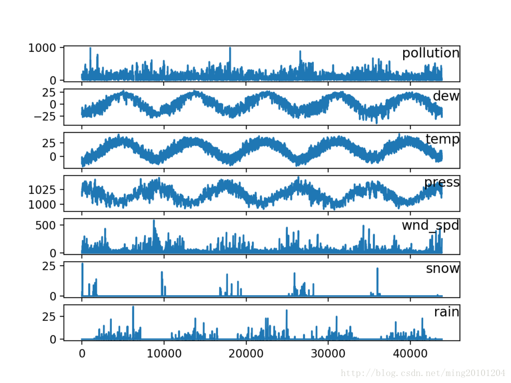
2010-01-02 04:00:00 138.0 -7 -5.0 1022.0 SE 6.25 2 0下面的代码加载了“pollution.csv”文件,并将每个列作为单独的子图绘制,除了风速dir,这是分类的。
from pandas import read_csv
from matplotlib import pyplot
# load dataset
dataset = read_csv('pollution.csv', header=0, index_col=0)
values = dataset.values
# specify columns to plot
groups = [0, 1, 2, 3, 5, 6, 7]
i = 1
# plot each column
pyplot.figure()
for group in groups:
    pyplot.subplot(len(groups), 1, i)
    pyplot.plot(values[:, group])
    pyplot.title(dataset.columns[group], y=0.5, loc='right')
    i += 1
pyplot.show()
运行示例创建7个子图,显示每个变量的5年数据。
Multivariate LSTM Forecast Model
在本节中,我们将适合LSTM的问题。
LSTM数据准备
第一步是为LSTM准备污染数据集。
这涉及将数据集视为监督学习问题并对输入变量进行归一化。
考虑到上一个时间段的污染测量和天气条件,我们将把监督学习问题作为预测当前时刻(t)的污染情况。
这个表述是直接的,只是为了这个演示。 您可以探索的一些替代配方包括:
根据过去24小时的天气情况和污染,预测下一个小时的污染。
预测下一个小时的污染,并给予下一个小时的“预期”天气条件。
我们可以使用在博客文章中开发的series_to_supervised()函数来转换数据集:
首先,加载“pollution.csv”数据集。 风速特征是标签编码(整数编码)。 如果您有兴趣探索,这可能会在将来进一步被热编码。
接下来,所有功能都被规范化,然后将数据集转换为监督学习问题。 然后删除要预测的小时的天气变量(t)。
完整的代码清单如下。
# convert series to supervised learning
def series_to_supervised(data, n_in=1, n_out=1, dropnan=True):
    n_vars = 1 if type(data) is list else data.shape[1]
    df = DataFrame(data)
    cols, names = list(), list()
    # input sequence (t-n, ... t-1)
    for i in range(n_in, 0, -1):
        cols.append(df.shift(i))
        names += [('var%d(t-%d)' % (j+1, i)) for j in range(n_vars)]
    # forecast sequence (t, t+1, ... t+n)
    for i in range(0, n_out):
        cols.append(df.shift(-i))
        if i == 0:
            names += [('var%d(t)' % (j+1)) for j in range(n_vars)]
        else:
            names += [('var%d(t+%d)' % (j+1, i)) for j in range(n_vars)]
    # put it all together
    agg = concat(cols, axis=1)
    agg.columns = names
    # drop rows with NaN values
    if dropnan:
        agg.dropna(inplace=True)
    return agg

# load dataset
dataset = read_csv('pollution.csv', header=0, index_col=0)
values = dataset.values
# integer encode direction
encoder = LabelEncoder()
values[:,4] = encoder.fit_transform(values[:,4])
# ensure all data is float
values = values.astype('float32')
# normalize features
scaler = MinMaxScaler(feature_range=(0, 1))
scaled = scaler.fit_transform(values)
# frame as supervised learning
reframed = series_to_supervised(scaled, 1, 1)
# drop columns we don't want to predict
reframed.drop(reframed.columns[[9,10,11,12,13,14,15]], axis=1, inplace=True)
print(reframed.head())
运行示例打印转换后的数据集的前5行。 我们可以看到8个输入变量(输入序列)和1个输出变量(当前小时的污染水平)。
   var1(t-1)  var2(t-1)  var3(t-1)  var4(t-1)  var5(t-1)  var6(t-1)  \
1   0.129779   0.352941   0.245902   0.527273   0.666667   0.002290
2   0.148893   0.367647   0.245902   0.527273   0.666667   0.003811
3   0.159960   0.426471   0.229508   0.545454   0.666667   0.005332
4   0.182093   0.485294   0.229508   0.563637   0.666667   0.008391
5   0.138833   0.485294   0.229508   0.563637   0.666667   0.009912

   var7(t-1)  var8(t-1)   var1(t)
1   0.000000        0.0  0.148893
2   0.000000        0.0  0.159960
3   0.000000        0.0  0.182093
4   0.037037        0.0  0.138833
5   0.074074        0.0  0.109658
这个数据准备很简单,我们可以探索更多。 您可以看到的一些想法包括:
单风编码风速。
使所有列均匀分散和季节性调整。
提供超过1小时的输入时间步长。
最后一点可能是最重要的,因为在学习序列预测问题时,LSTMs通过时间使用反向传播。
Define and Fit Model
在本节中,我们将适合多变量输入数据的LSTM。
首先,我们必须将准备好的数据集分成训练集和测试集。 为了加快对模型快速拟合,我们将仅适用于数据第一年的模型,然后对其余4年的数据进行评估。
下面的示例将数据集分成训练集和测试集,然后将训练集和测试集分成输入和输出变量。 最后,将输入(X)重构为LSTM预期的3D格式,即[样本,时间步长,特征]。
# split into train and test sets
values = reframed.values
n_train_hours = 365 * 24
train = values[:n_train_hours, :]
test = values[n_train_hours:, :]
# split into input and outputs
train_X, train_y = train[:, :-1], train[:, -1]
test_X, test_y = test[:, :-1], test[:, -1]
# reshape input to be 3D [samples, timesteps, features]
train_X = train_X.reshape((train_X.shape[0], 1, train_X.shape[1]))
test_X = test_X.reshape((test_X.shape[0], 1, test_X.shape[1]))
print(train_X.shape, train_y.shape, test_X.shape, test_y.shape)
运行此示例打印训练集的形状,并测试输入和输出集合约9K小时的数据进行培训,约35K小时进行测试。
(8760, 1, 8) (8760,) (35039, 1, 8) (35039,)现在我们可以定义和fit我们的LSTM模型。
我们将在第一个隐层中定义具有50个神经元的LSTM和用于预测污染的输出层中的1个神经元。 输入形状将是1个时间步长,具有8个特征。
我们将使用平均绝对误差(MAE)损失函数和Adam中的随机梯度下降。
该模型将适合50个批量大小为72的训练时期。请记住,每个批次结束时,Keras中的LSTM的内部状态都将重置,因此内部状态是多少天的函数对此有帮助(尝试测试这个)。
最后,我们通过在fit()函数中设置validation_data参数来跟踪训练过程中的训练和测试失败。 在运行结束时,绘制训练和测试损失。
# design network
model = Sequential()
model.add(LSTM(50, input_shape=(train_X.shape[1], train_X.shape[2])))
model.add(Dense(1))
model.compile(loss='mae', optimizer='adam')
# fit network
history = model.fit(train_X, train_y, epochs=50, batch_size=72, validation_data=(test_X, test_y), verbose=2, shuffle=False)
# plot history
pyplot.plot(history.history['loss'], label='train')
pyplot.plot(history.history['val_loss'], label='test')
pyplot.legend()
pyplot.show()
Evaluate Model
模型fit后,我们可以预测整个测试数据集。
我们将预测与测试数据集相结合,并反演缩放。 我们还用预期的污染数字来反演测试数据集的缩放。
以预测值和实际值为原始尺度,我们可以计算模型的误差分数。 在这种情况下,我们计算出与变量本身相同的单位产生误差的均方根误差(RMSE)。
# make a prediction
yhat = model.predict(test_X)
test_X = test_X.reshape((test_X.shape[0], test_X.shape[2]))
# invert scaling for forecast
inv_yhat = concatenate((yhat, test_X[:, 1:]), axis=1)
inv_yhat = scaler.inverse_transform(inv_yhat)
inv_yhat = inv_yhat[:,0]
# invert scaling for actual
inv_y = scaler.inverse_transform(test_X)
inv_y = inv_y[:,0]
# calculate RMSE
rmse = sqrt(mean_squared_error(inv_y, inv_yhat))
print('Test RMSE: %.3f' % rmse)
Complete Example
完整的示例如下所示。
from math import sqrt
from numpy import concatenate
from matplotlib import pyplot
from pandas import read_csv
from pandas import DataFrame
from pandas import concat
from sklearn.preprocessing import MinMaxScaler
from sklearn.preprocessing import LabelEncoder
from sklearn.metrics import mean_squared_error
from keras.models import Sequential
from keras.layers import Dense
from keras.layers import LSTM

# convert series to supervised learning
def series_to_supervised(data, n_in=1, n_out=1, dropnan=True):
    n_vars = 1 if type(data) is list else data.shape[1]
    df = DataFrame(data)
    cols, names = list(), list()
    # input sequence (t-n, ... t-1)
    for i in range(n_in, 0, -1):
        cols.append(df.shift(i))
        names += [('var%d(t-%d)' % (j+1, i)) for j in range(n_vars)]
    # forecast sequence (t, t+1, ... t+n)
    for i in range(0, n_out):
        cols.append(df.shift(-i))
        if i == 0:
            names += [('var%d(t)' % (j+1)) for j in range(n_vars)]
        else:
            names += [('var%d(t+%d)' % (j+1, i)) for j in range(n_vars)]
    # put it all together
    agg = concat(cols, axis=1)
    agg.columns = names
    # drop rows with NaN values
    if dropnan:
        agg.dropna(inplace=True)
    return agg

# load dataset
dataset = read_csv('pollution.csv', header=0, index_col=0)
values = dataset.values
# integer encode direction
encoder = LabelEncoder()
values[:,4] = encoder.fit_transform(values[:,4])
# ensure all data is float
values = values.astype('float32')
# normalize features
scaler = MinMaxScaler(feature_range=(0, 1))
scaled = scaler.fit_transform(values)
# frame as supervised learning
reframed = series_to_supervised(scaled, 1, 1)
# drop columns we don't want to predict
reframed.drop(reframed.columns[[9,10,11,12,13,14,15]], axis=1, inplace=True)
print(reframed.head())

# split into train and test sets
values = reframed.values
n_train_hours = 365 * 24
train = values[:n_train_hours, :]
test = values[n_train_hours:, :]
# split into input and outputs
train_X, train_y = train[:, :-1], train[:, -1]
test_X, test_y = test[:, :-1], test[:, -1]
# reshape input to be 3D [samples, timesteps, features]
train_X = train_X.reshape((train_X.shape[0], 1, train_X.shape[1]))
test_X = test_X.reshape((test_X.shape[0], 1, test_X.shape[1]))
print(train_X.shape, train_y.shape, test_X.shape, test_y.shape)

# design network
model = Sequential()
model.add(LSTM(50, input_shape=(train_X.shape[1], train_X.shape[2])))
model.add(Dense(1))
model.compile(loss='mae', optimizer='adam')
# fit network
history = model.fit(train_X, train_y, epochs=50, batch_size=72, validation_data=(test_X, test_y), verbose=2, shuffle=False)
# plot history
pyplot.plot(history.history['loss'], label='train')
pyplot.plot(history.history['val_loss'], label='test')
pyplot.legend()
pyplot.show()

# make a prediction
yhat = model.predict(test_X)
test_X = test_X.reshape((test_X.shape[0], test_X.shape[2]))
# invert scaling for forecast
inv_yhat = concatenate((yhat, test_X[:, 1:]), axis=1)
inv_yhat = scaler.inverse_transform(inv_yhat)
inv_yhat = inv_yhat[:,0]
# invert scaling for actual
inv_y = scaler.inverse_transform(test_X)
inv_y = inv_y[:,0]
# calculate RMSE
rmse = sqrt(mean_squared_error(inv_y, inv_yhat))
print('Test RMSE: %.3f' % rmse)
运行示例首先创建一个绘图,显示培训中的训练集和测试集损失。
有趣的是,我们可以看到测试损失低于训练损失。 该模型可能过度拟合训练数据。 在训练过程中测量和绘制RMSE。
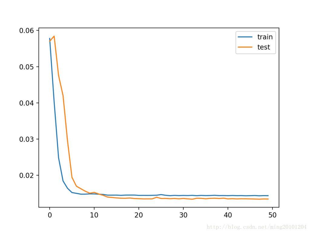
训练和测试损失在每个训练期结束后打印。 在运行结束时,打印测试数据集上模型的最终RMSE。
我们可以看到,该模型实现了3.836的可观RMSE,这显著低于用持续模型发现的RMSE的30。
...
Epoch 46/50
0s - loss: 0.0143 - val_loss: 0.0133
Epoch 47/50
0s - loss: 0.0143 - val_loss: 0.0133
Epoch 48/50
0s - loss: 0.0144 - val_loss: 0.0133
Epoch 49/50
0s - loss: 0.0143 - val_loss: 0.0133
Epoch 50/50
0s - loss: 0.0144 - val_loss: 0.0133
Test RMSE: 3.836
这个模型没有调参。 你能做得更好吗?
让我在下面的评论中知道您的问题框架,模型配置和RMSE。