边学习边笔记
https://www.cnblogs.com/felixwang2/p/9190602.html


  1 # https://www.cnblogs.com/felixwang2/p/9190602.html
  2 # TensorFlow(十):卷积神经网络实现手写数字识别以及可视化
  3
  4 import tensorflow as tf
  5 from tensorflow.examples.tutorials.mnist import input_data
  6
  7 mnist = input_data.read_data_sets('MNIST_data', one_hot=True)
  8
  9 # 每个批次的大小
 10 batch_size = 100
 11 # 计算一共有多少个批次
 12 n_batch = mnist.train.num_examples // batch_size
 13
 14
 15 # 参数概要
 16 def variable_summaries(var):
 17     with tf.name_scope('summaries'):
 18         mean = tf.reduce_mean(var)
 19         tf.summary.scalar('mean', mean)  # 平均值
 20         with tf.name_scope('stddev'):
 21             stddev = tf.sqrt(tf.reduce_mean(tf.square(var - mean)))
 22         tf.summary.scalar('stddev', stddev)  # 标准差
 23         tf.summary.scalar('max', tf.reduce_max(var))  # 最大值
 24         tf.summary.scalar('min', tf.reduce_min(var))  # 最小值
 25         tf.summary.histogram('histogram', var)  # 直方图
 26
 27
 28 # 初始化权值
 29 def weight_variable(shape, name):
 30     initial = tf.truncated_normal(shape, stddev=0.1)  # 生成一个截断的正态分布
 31     return tf.Variable(initial, name=name)
 32
 33
 34 # 初始化偏置
 35 def bias_variable(shape, name):
 36     initial = tf.constant(0.1, shape=shape)
 37     return tf.Variable(initial, name=name)
 38
 39
 40 # 卷积层
 41 def conv2d(x, W):
 42     # x input tensor of shape `[batch, in_height, in_width, in_channels]`
 43     # W filter / kernel tensor of shape [filter_height, filter_width, in_channels, out_channels]
 44     # `strides[0] = strides[3] = 1`. strides[1]代表x方向的步长,strides[2]代表y方向的步长
 45     # padding: A `string` from: `"SAME", "VALID"`
 46     return tf.nn.conv2d(x, W, strides=[1, 1, 1, 1], padding='SAME')
 47
 48
 49 # 池化层
 50 def max_pool_2x2(x):
 51     # ksize [1,x,y,1]
 52     return tf.nn.max_pool(x, ksize=[1, 2, 2, 1], strides=[1, 2, 2, 1], padding='SAME')
 53
 54
 55 # 命名空间
 56 with tf.name_scope('input'):
 57     # 定义两个placeholder
 58     x = tf.placeholder(tf.float32, [None, 784], name='x-input')
 59     y = tf.placeholder(tf.float32, [None, 10], name='y-input')
 60     with tf.name_scope('x_image'):
 61         # 改变x的格式转为4D的向量[batch, in_height, in_width, in_channels]`
 62         x_image = tf.reshape(x, [-1, 28, 28, 1], name='x_image')
 63
 64 with tf.name_scope('Conv1'):
 65     # 初始化第一个卷积层的权值和偏置
 66     with tf.name_scope('W_conv1'):
 67         W_conv1 = weight_variable([5, 5, 1, 32], name='W_conv1')  # 5*5的采样窗口,32个卷积核从1个平面抽取特征
 68     with tf.name_scope('b_conv1'):
 69         b_conv1 = bias_variable([32], name='b_conv1')  # 每一个卷积核一个偏置值
 70
 71     # 把x_image和权值向量进行卷积,再加上偏置值,然后应用于relu激活函数
 72     with tf.name_scope('conv2d_1'):
 73         conv2d_1 = conv2d(x_image, W_conv1) + b_conv1
 74     with tf.name_scope('relu'):
 75         h_conv1 = tf.nn.relu(conv2d_1)
 76     with tf.name_scope('h_pool1'):
 77         h_pool1 = max_pool_2x2(h_conv1)  # 进行max-pooling
 78
 79 with tf.name_scope('Conv2'):
 80     # 初始化第二个卷积层的权值和偏置
 81     with tf.name_scope('W_conv2'):
 82         W_conv2 = weight_variable([5, 5, 32, 64], name='W_conv2')  # 5*5的采样窗口,64个卷积核从32个平面抽取特征
 83     with tf.name_scope('b_conv2'):
 84         b_conv2 = bias_variable([64], name='b_conv2')  # 每一个卷积核一个偏置值
 85
 86     # 把h_pool1和权值向量进行卷积,再加上偏置值,然后应用于relu激活函数
 87     with tf.name_scope('conv2d_2'):
 88         conv2d_2 = conv2d(h_pool1, W_conv2) + b_conv2
 89     with tf.name_scope('relu'):
 90         h_conv2 = tf.nn.relu(conv2d_2)
 91     with tf.name_scope('h_pool2'):
 92         h_pool2 = max_pool_2x2(h_conv2)  # 进行max-pooling
 93
 94 # 28*28的图片第一次卷积后还是28*28,第一次池化后变为14*14
 95 # 第二次卷积后为14*14,第二次池化后变为了7*7
 96 # 经过上面操作后得到64张7*7的平面
 97
 98 with tf.name_scope('fc1'):
 99     # 初始化第一个全连接层的权值
100     with tf.name_scope('W_fc1'):
101         W_fc1 = weight_variable([7 * 7 * 64, 1024], name='W_fc1')  # 上一场有7*7*64个神经元,全连接层有1024个神经元
102     with tf.name_scope('b_fc1'):
103         b_fc1 = bias_variable([1024], name='b_fc1')  # 1024个节点
104
105     # 把池化层2的输出扁平化为1维
106     with tf.name_scope('h_pool2_flat'):
107         h_pool2_flat = tf.reshape(h_pool2, [-1, 7 * 7 * 64], name='h_pool2_flat')
108     # 求第一个全连接层的输出
109     with tf.name_scope('wx_plus_b1'):
110         wx_plus_b1 = tf.matmul(h_pool2_flat, W_fc1) + b_fc1
111     with tf.name_scope('relu'):
112         h_fc1 = tf.nn.relu(wx_plus_b1)
113
114     # keep_prob用来表示神经元的输出概率
115     with tf.name_scope('keep_prob'):
116         keep_prob = tf.placeholder(tf.float32, name='keep_prob')
117     with tf.name_scope('h_fc1_drop'):
118         h_fc1_drop = tf.nn.dropout(h_fc1, keep_prob, name='h_fc1_drop')
119
120 with tf.name_scope('fc2'):
121     # 初始化第二个全连接层
122     with tf.name_scope('W_fc2'):
123         W_fc2 = weight_variable([1024, 10], name='W_fc2')
124     with tf.name_scope('b_fc2'):
125         b_fc2 = bias_variable([10], name='b_fc2')
126     with tf.name_scope('wx_plus_b2'):
127         wx_plus_b2 = tf.matmul(h_fc1_drop, W_fc2) + b_fc2
128     with tf.name_scope('softmax'):
129         # 计算输出
130         prediction = tf.nn.softmax(wx_plus_b2)
131
132 # 交叉熵代价函数
133 with tf.name_scope('cross_entropy'):
134     cross_entropy = tf.reduce_mean(tf.nn.softmax_cross_entropy_with_logits_v2(labels=y, logits=prediction),
135                                    name='cross_entropy')
136     tf.summary.scalar('cross_entropy', cross_entropy)
137
138 # 使用AdamOptimizer进行优化
139 with tf.name_scope('train'):
140     train_step = tf.train.AdamOptimizer(1e-4).minimize(cross_entropy)
141
142 # 求准确率
143 with tf.name_scope('accuracy'):
144     with tf.name_scope('correct_prediction'):
145         # 结果存放在一个布尔列表中
146         correct_prediction = tf.equal(tf.argmax(prediction, 1), tf.argmax(y, 1))  # argmax返回一维张量中最大的值所在的位置
147     with tf.name_scope('accuracy'):
148         # 求准确率
149         accuracy = tf.reduce_mean(tf.cast(correct_prediction, tf.float32))
150         tf.summary.scalar('accuracy', accuracy)
151
152 # 合并所有的summary
153 merged = tf.summary.merge_all()
154
155 gpu_options = tf.GPUOptions(allow_growth=True)
156 with tf.Session(config=tf.ConfigProto(gpu_options=gpu_options)) as sess:
157     sess.run(tf.global_variables_initializer())
158     train_writer = tf.summary.FileWriter('logs/train', sess.graph)
159     test_writer = tf.summary.FileWriter('logs/test', sess.graph)
160     for i in range(1001):
161         # 训练模型
162         batch_xs, batch_ys = mnist.train.next_batch(batch_size)
163         sess.run(train_step, feed_dict={x: batch_xs, y: batch_ys, keep_prob: 0.5})
164         # 记录训练集计算的参数
165         summary = sess.run(merged, feed_dict={x: batch_xs, y: batch_ys, keep_prob: 1.0})
166         train_writer.add_summary(summary, i)
167         # 记录测试集计算的参数
168         batch_xs, batch_ys = mnist.test.next_batch(batch_size)
169         summary = sess.run(merged, feed_dict={x: batch_xs, y: batch_ys, keep_prob: 1.0})
170         test_writer.add_summary(summary, i)
171
172         if i % 100 == 0:
173             test_acc = sess.run(accuracy, feed_dict={x: mnist.test.images, y: mnist.test.labels, keep_prob: 1.0})
174             train_acc = sess.run(accuracy, feed_dict={x: mnist.train.images[:10000], y: mnist.train.labels[:10000],
175                                                       keep_prob: 1.0})
176             print("Iter " + str(i) + ", Testing Accuracy= " + str(test_acc) + ", Training Accuracy= " + str(train_acc))
应该是随便在某个路径下,右键,打开powershell窗口,输入如下命令:
tensorboard --logdir=F:\document\PyCharm\temp\logs
之后会在窗口输出:
TensorBoard 1.10.0 at http://KOTIN:6006 (Press CTRL+C to quit)
然后在浏览器输入
http://KOTIN:6006
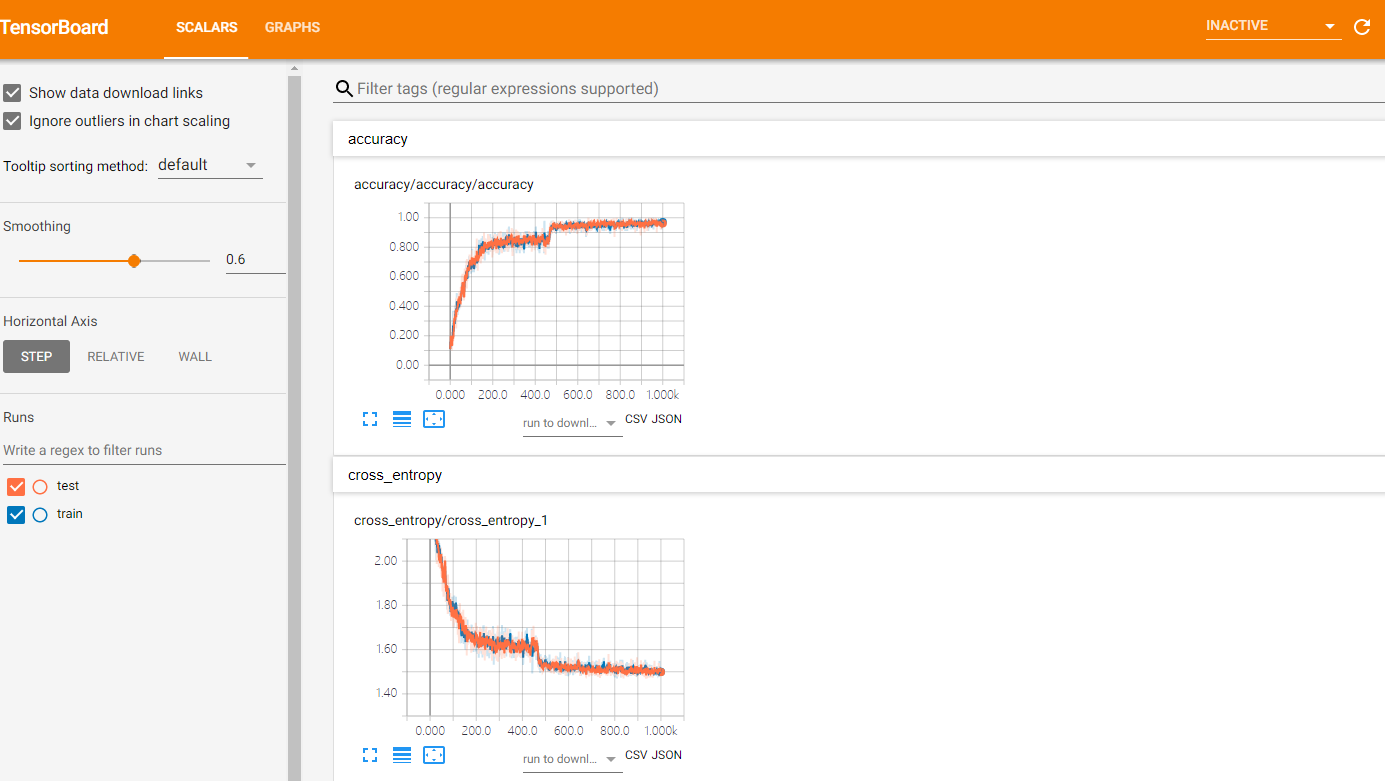
就可以进入tensorboard查看参数的可视化信息: