普通神经网络与卷积神经网络手写数字识别对比------基于tensorflow

前言

今天上午花了几个小时的时间把电脑清理了一下，把anaconda、tensorflow-gpu等东西都重新安装了一遍，现在电脑可以用GPU来跑这些神经网络的代码了。下面开始介绍：
关于神经网络和卷积神经网络的内容，我并不觉得我能比CSDN的大佬讲得更好，所以我直接跳过这方面的介绍直接展示代码并讲解，如果对相关的知识了解的不够全面可以参考一下下面的两篇博客（ps:我觉得讲的还挺好的）：
神经网络（入门最详细）
CNN笔记：通俗理解卷积神经网络
也可以尝试看看我之前有做过的：
基于CNN的象棋棋子识别

数据集

手写数字数据集，对于入门机器学习的童鞋来说应该是接触的最早的几个数据集之一了，这是下载网址：http://yann.lecun.com/exdb/mnist/.
当然，其实没有必要去访问这个网站，直接可以用代码去下载调用。

---

MNIST数据集是由0到9的数字图像构成的。训练图像有6万张，测试图像有1万张。MNIST数据集是NIST数据集的一个子集，它包含了60000张图片作为训练数据，10000张图片作为测试数据。由250个不同的人手写而成。

每一张图片都有对应的标签数字，训练图像一共有60000 张，供研究人员训练出合适的模型。测试图像一共有10000 张，供研究人员测试训练的模型的性能。

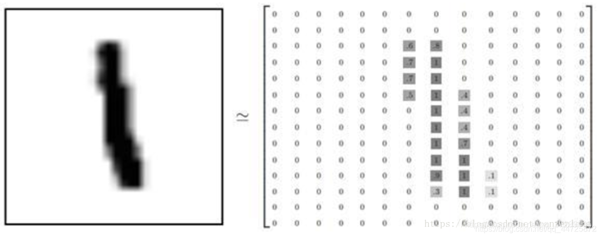
这些手写图片都是2828像素，灰度图像。

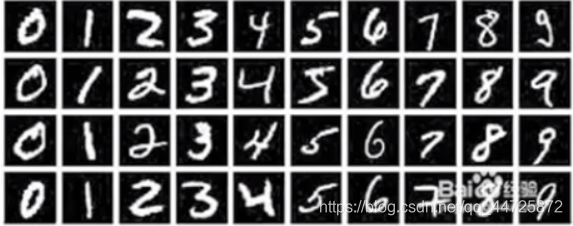
但是它们并不是作为图像文件存储的，而是2828的二维数组中。数组中的每个元素对应数组中的每个像素。

原文链接：手写数字数据集MNIST
这篇博客里有写直接用keras调用，但是我没用这种方法。我直接用的从网上找到的mnist的input_data文件，然后直接导入程序文件里进行使用。如有需要可以直接将下面博客里的代码保存为一个input_data.py的文件放到程序文件同级目录下。Mnist数据集以及input_data.py的代码

代码

编程环境：VS code、Tensorflow-gpu-2.4.1

普通神经网络

回归正题，首先我们来看看基于tensorflow的神经网络代码，代码源于书本—《Fundamentals of deep learning》
模型结构：输入层—第一隐藏层—第二隐藏层—输出层

import tensorflow.compat.v1 as tf
import input_data



#网络结构定义
#定义层
def layer(_input_, weight_shape, bias_shape):
    weight_stddev = (2.0 /  weight_shape[0]) ** 0.5
    weights_init = tf.random_normal_initializer(stddev=weight_stddev)
    bias_init = tf.constant_initializer(value=0.0,dtype=tf.float32)
    w = tf.get_variable("W",weight_shape,
                        initializer=weights_init)
    b = tf.get_variable("b",bias_shape,
                        initializer=bias_init)
    return tf.nn.relu(tf.matmul(_input_,w) + b)
#
#定义网络
def inference(x):
    with tf.variable_scope("hidden_1"):
        #第一隐藏层
        hidden_1 = layer(x,[784,256],[256])
    with tf.variable_scope("hidden_2"):
        #第二隐藏层
        hidden_2 = layer(hidden_1,[256,256],[256])
    with tf.variable_scope("output"):
        #输出层
        weight_stddev = (2.0 / 256) ** 0.5
        weights_init = tf.random_normal_initializer(stddev=weight_stddev)
        bias_init = tf.constant_initializer(value=0.0,dtype=tf.float32)
        W = tf.get_variable("W",dtype=tf.float32,shape=[256,10],initializer=weights_init)
        b = tf.get_variable("b",dtype=tf.float32,shape=[10],initializer=bias_init)
        logits = tf.matmul(hidden_2,W) + b
        output = tf.nn.softmax(logits)

    return output

#损失函数
def loss(output,y):
    dot_product = y * tf.log(output)
    xentropy = -tf.reduce_sum(dot_product,reduction_indices=1)
    loss = tf.reduce_mean(xentropy)

    return loss
#

#训练函数
def training(cost,global_step):
    tf.summary.scalar("cost",cost)#################
    optimizer = tf.train.GradientDescentOptimizer(learning_rate)
    train_op = optimizer.minimize(cost,global_step=global_step)

    return train_op
#

#计算accuracy
def evaluate(output,y):
    correct_prediction = tf.equal(tf.argmax(output,1),
                                    tf.argmax(y,1))
    accuracy = tf.reduce_mean(tf.cast(correct_prediction,tf.float32))

    return accuracy
#

#宏参数
learning_rate = 0.01
training_epochs = 50
batch_size = 100
display_step = 1
#

#数据源
mnist = input_data.read_data_sets('MNIST_data',one_hot=True)
#

#空出一定量的GPU空间
gpu_options = tf.GPUOptions(per_process_gpu_memory_fraction=0.8)
#

tf.disable_eager_execution()
with tf.Graph().as_default():
    #输入的数据，28*28
    x = tf.placeholder("float",[None,784])

    #输出数据，10个分类的概率分布
    y = tf.placeholder("float",[None,10])

    output = inference(x)

    cost = loss(output,y)

    global_step = tf.Variable(0,name='global_step',trainable=False)

    train_op = training(cost,global_step)

    eval_op = evaluate(output,y)

    summary_op = tf.summary.merge_all()#######################
    saver = tf.train.Saver()################


    sess = tf.Session(config=tf.ConfigProto(gpu_options=gpu_options))

    summary_writer = tf.summary.FileWriter("logistic_logs/",
                                            graph_def=sess.graph_def)####

    init_op = tf.global_variables_initializer()

    sess.run(init_op)

    #开始训练
    for epoch in range(training_epochs):

        avg_cost = 0
        total_batch = int(mnist.train.num_examples/batch_size)
        #循环处理所有批
        for i in range(total_batch):
            mbatch_x,mbatch_y = mnist.train.next_batch(batch_size)

            feed_dict = {
    
    x:mbatch_x,y:mbatch_y}
            sess.run(train_op,feed_dict=feed_dict)
            #计算平均损失
            minibatch_cost = sess.run(cost,feed_dict=feed_dict)
            avg_cost += minibatch_cost/total_batch

        if epoch % display_step == 0:
            val_feed_dict = {
    
    
                x:mnist.validation.images,
                y:mnist.validation.labels
            }
            accuracy = sess.run(eval_op,feed_dict=val_feed_dict)
            print("Validation Error:",(1-accuracy))

            summary_str = sess.run(summary_op,feed_dict=feed_dict)#######
            summary_writer.add_summary(summary_str,sess.run(global_step))########
            saver.save(sess,"logistic_logs/model-checkpoint",global_step=global_step)####

    print("Optimization Finished!")
    test_feed_dict = {
    
    
        x:mnist.test.images,
        y:mnist.test.labels
    }
    accuracy = sess.run(eval_op,feed_dict=test_feed_dict)
    print("Test Accuracy:",accuracy)

10次迭代下普通的神经网络的结果表现的不太行，测试集的准确率只有94.34%，一些其他的算法（例如支持向量机）的表现都可能超过这个。

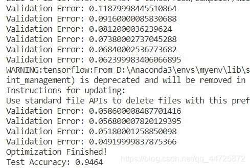
当然了，这里也只是迭代了10次，为了控制时间所以和下面的卷积神经网络的迭代次数是一样的。如果将迭代次数升高，也有可能得到下面的结果：

98.02%，是将迭代次数增加到100后的结果，但是耗费的时间已经快超过下面的卷积神经网络的耗时了。

卷积神经网络

模型结构：卷积层—卷积层—最大池化层—Flatten层—全连接层—输出

import numpy as np
import keras
from keras.models import Sequential
from keras.layers import Dense, Dropout, Flatten
from keras.layers import Conv2D, MaxPooling2D
import os
import warnings
import input_data
# 忽略硬件加速的警告信息
os.environ['TF_CPP_MIN_LOG_LEVEL'] = '2'
warnings.filterwarnings('ignore')

mnist = input_data.read_data_sets('MNIST_data',one_hot=True)


#batch_size=50    #每次喂给网络50组数据
#*********************************************************************************************************************************************#
#卷积神经网络模型，采用keras进行搭建
model = Sequential() #这里使用序贯模型，比较容易理解,序贯模型就像搭积木一样，将神经网络一层一层往上搭上去
#搭一个卷积层
model.add(Conv2D(28, (3,3), activation='relu', padding='same', data_format='channels_last',name='layer1_con1',input_shape=(28,28,1)))
#再搭一层卷积层
model.add(Conv2D(28, (3,3), activation='relu', padding='same', data_format='channels_last',name='layer1_con2'))
#搭一个最大池化层
model.add(MaxPooling2D(pool_size=(2, 2),strides=(2,2), padding = 'same', data_format='channels_last',name = 'layer1_pool'))

model.add(Flatten())
model.add(Dense(64, activation='relu'))  #该全连接层共128个神经元
model.add(Dense(10, activation='softmax')) #一共分为10类，所以最后一层有10个神经元，并且采用softmax输出
model.compile(loss='categorical_crossentropy', optimizer='adam', metrics = ['accuracy'])#定义损失值、优化器
#*********************************************************************************************************************************************#

#训练
X_train = mnist.train.images.reshape(55000,28,28,1)
y_train = mnist.train.labels
model.fit(X_train, y_train,epochs=10,batch_size=100)

#计算得分
X_test = mnist.test.images.reshape(10000,28,28,1)
y_test = mnist.test.labels
[loss,accuracy] = model.evaluate(X_test, y_test)
print('\nTest Loss: ', loss)
print('\nTest Accuracy: ', accuracy)
#保存模型,
model.save("model_new.h5")
#*********************************************************************************************************************************************#

这里的卷积神经网络模型是用我前面提到的博客里的模型删掉一部分改的，所以可能并不太适合于这个数据集，最终结果比我之前看到的别人写的要菜一点。下面是结果，10次迭代：

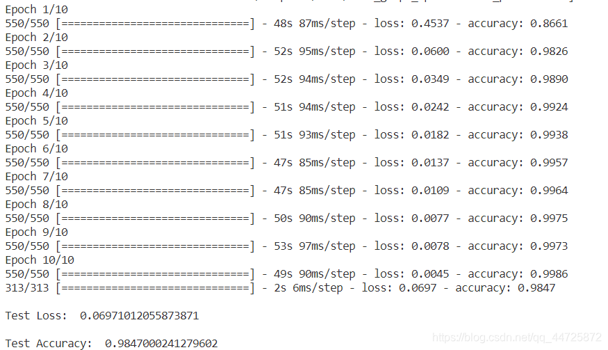
可以看到训练集的准确率已经到达99.86%了，测试集的结果也有98.47%。

终末

通过上面的比较，显而易见在手写数字识别上，卷积神经网络的表现要远远优于普通的神经网络。因为笔者平时也有接触，卷积神经网络其实在大多数的图像识别上表现得都非常优秀，现在的用途也十分广泛。
但我在跑这俩模型的时候，不知道是卷积神经网络本身模型的问题（ps：理论上分析卷积神经网络的训练速度应该是要比普通的神经网络要快很多的）还是keras封装后的问题亦或者我的笔记本的显卡过于垃圾，上面两个模型的训练速度相差甚大，普通神经网络花了一分钟多点，但卷积神经网络花了超过五分钟。