上一篇博客中,我们已经训练好了模型
https://blog.csdn.net/Polaris47/article/details/80718328
接下来我们要加载模型并识别真实场景下的一个手写体数字
在此之前,我们先要准备好一张28*28像素的图像(可用ps制作),然后通过处理将像素的强度值变为0-1之间,之后即可输入模型进行识别。
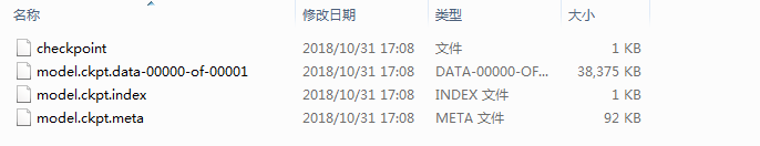
保存已训练的模型文件如下:
代码如下:
import tensorflow as tf
import matplotlib.pyplot as plt
from PIL import Image
def imageprepare(imagepath):
im = Image.open(imagepath) #读取的图片所在路径,注意是28*28像素
plt.imshow(im) #显示需要识别的图片
plt.show()
im = im.convert('L')
tv = list(im.getdata())
tva = [(255-x)*1.0/255.0 for x in tv]
return tva
def weight_variable(shape, name):
initial = tf.truncated_normal(shape, stddev=0.1) # 生成一个截断的正态分布
return tf.Variable(initial, name=name)
# 初始化偏置
def bias_variable(shape, name):
initial = tf.constant(0.1, shape=shape)
return tf.Variable(initial, name=name)
# 卷积层
def conv2d(x, W):
# x input tensor of shape `[batch, in_height, in_width, in_channels]`
# W filter / kernel tensor of shape [filter_height, filter_width, in_channels, out_channels]
# `strides[0] = strides[3] = 1`. strides[1]代表x方向的步长,strides[2]代表y方向的步长
# padding: A `string` from: `"SAME", "VALID"`
return tf.nn.conv2d(x, W, strides=[1, 1, 1, 1], padding='SAME')
# 池化层
def max_pool_2x2(x):
# ksize [1,x,y,1]
return tf.nn.max_pool(x, ksize=[1, 2, 2, 1], strides=[1, 2, 2, 1], padding='SAME')
# 命名空间
with tf.name_scope('input'):
# 定义两个placeholder
x = tf.placeholder(tf.float32, [None, 784], name='x-input')
y = tf.placeholder(tf.float32, [None, 10], name='y-input')
with tf.name_scope('x_image'):
# 改变x的格式转为4D的向量[batch, in_height, in_width, in_channels]`
x_image = tf.reshape(x, [-1, 28, 28, 1], name='x_image')
with tf.name_scope('Conv1'):
# 初始化第一个卷积层的权值和偏置
with tf.name_scope('W_conv1'):
W_conv1 = weight_variable([5, 5, 1, 32], name='W_conv1') # 5*5的采样窗口,32个卷积核从1个平面抽取特征
with tf.name_scope('b_conv1'):
b_conv1 = bias_variable([32], name='b_conv1') # 每一个卷积核一个偏置值
# 把x_image和权值向量进行卷积,再加上偏置值,然后应用于relu激活函数
with tf.name_scope('conv2d_1'):
conv2d_1 = conv2d(x_image, W_conv1) + b_conv1
with tf.name_scope('relu'):
h_conv1 = tf.nn.relu(conv2d_1)
with tf.name_scope('h_pool1'):
h_pool1 = max_pool_2x2(h_conv1) # 进行max-pooling
with tf.name_scope('Conv2'):
# 初始化第二个卷积层的权值和偏置
with tf.name_scope('W_conv2'):
W_conv2 = weight_variable([5, 5, 32, 64], name='W_conv2') # 5*5的采样窗口,64个卷积核从32个平面抽取特征
with tf.name_scope('b_conv2'):
b_conv2 = bias_variable([64], name='b_conv2') # 每一个卷积核一个偏置值
# 把h_pool1和权值向量进行卷积,再加上偏置值,然后应用于relu激活函数
with tf.name_scope('conv2d_2'):
conv2d_2 = conv2d(h_pool1, W_conv2) + b_conv2
with tf.name_scope('relu'):
h_conv2 = tf.nn.relu(conv2d_2)
with tf.name_scope('h_pool2'):
h_pool2 = max_pool_2x2(h_conv2) # 进行max-pooling
# 28*28的图片第一次卷积后还是28*28,第一次池化后变为14*14
# 第二次卷积后为14*14,第二次池化后变为了7*7
# 进过上面操作后得到64张7*7的平面
with tf.name_scope('fc1'):
# 初始化第一个全连接层的权值
with tf.name_scope('W_fc1'):
W_fc1 = weight_variable([7 * 7 * 64, 1024], name='W_fc1') # 上一场有7*7*64个神经元,全连接层有1024个神经元
with tf.name_scope('b_fc1'):
b_fc1 = bias_variable([1024], name='b_fc1') # 1024个节点
# 把池化层2的输出扁平化为1维
with tf.name_scope('h_pool2_flat'):
h_pool2_flat = tf.reshape(h_pool2, [-1, 7 * 7 * 64], name='h_pool2_flat')
# 求第一个全连接层的输出
with tf.name_scope('wx_plus_b1'):
wx_plus_b1 = tf.matmul(h_pool2_flat, W_fc1) + b_fc1
with tf.name_scope('relu'):
h_fc1 = tf.nn.relu(wx_plus_b1)
# keep_prob用来表示神经元的输出概率
with tf.name_scope('keep_prob'):
keep_prob = tf.placeholder(tf.float32, name='keep_prob')
with tf.name_scope('h_fc1_drop'):
h_fc1_drop = tf.nn.dropout(h_fc1, keep_prob, name='h_fc1_drop')
with tf.name_scope('fc2'):
# 初始化第二个全连接层
with tf.name_scope('W_fc2'):
W_fc2 = weight_variable([1024, 10], name='W_fc2')
with tf.name_scope('b_fc2'):
b_fc2 = bias_variable([10], name='b_fc2')
with tf.name_scope('wx_plus_b2'):
wx_plus_b2 = tf.matmul(h_fc1_drop, W_fc2) + b_fc2
with tf.name_scope('softmax'):
# 计算输出
prediction = tf.nn.softmax(wx_plus_b2)
res = tf.argmax(prediction, 1)
saver = tf.train.Saver()
image = imageprepare('6.png')
with tf.Session() as sess:
saver.restore(sess, "cnn_Model/model.ckpt")
result = sess.run(res,feed_dict={x: [image],keep_prob:1.0})
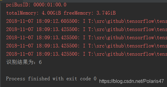
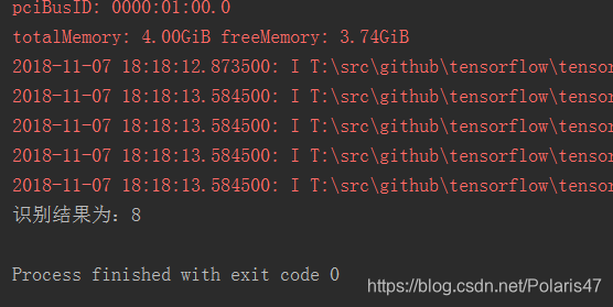
print('识别结果为:%d' %result)
制作的图像和识别结果如下: