Model-Based and Model-Free
In the previous several posts, we mainly talked about Model-Based Reinforcement Learning. The biggest assumption for Model-Based learning is the whole knowledge of the environment is given, but it is unrealistic in real life or even video games. I do believe unknown makes life (game) interesting. Personally, everytime I know what will happen in a game, I get rid of it! So, people like playing games with some uncertainties. That is what Model-Free Reinforcement Learning does: lean the unknown environment, and then come up with the best policy.
Two Task for Model-Free Learning
For Model-Based Learning,we have two tasks: Evaluation and Control. We use Dynamic Programming to evaluate a policy, while two algorithms called Policy Iteration and Value Iteration are used to extract the optimal policy. In Model-Free Learning, we have the same two tasks:
Evaluation: we need to estimate State-Value functions for every state, although Transition Matrices and Reward Function are not given.
Control: we need to find the best policy to solve the interesting game.
Monte Carlo Method in Daily Life
One of the algorithms for Evaluation is Monte Carlo Method. Probably the superior name 'Monte Carlo' is scaring, but you would feel comfortable while following my example below.
Assume our task is traveling from London to Toronto, and the policy is 'random walk'. we define travel distance and time as rewards. There are cities, towns, even villages on the map on which agents would randomly draw diverse trajectories from London to Toronto. Even it is possible that an agent arrives and departs some places more than once. But finally every agent will complete an episode when it arrives at Toronto, and then we can review paths, learning experience from trials.
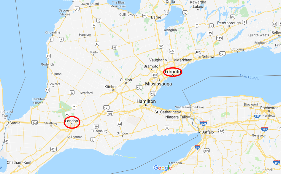
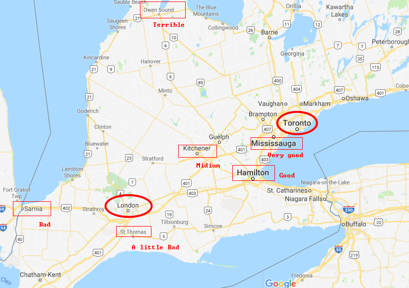
Finally, we will know goodnesses of being in every place on the map. Mississauga is a very good state for our task, but the state Owen Sound is terrible. The reason why we can get this conclusion is: states closed to the final state usually have great State-Value functions, because they tend to win the game soon. Episodes in our example that get to Mississauga have great probabilities getting to Toronto soon, so the Expectation of their State-Value functions is also high. On the other hand, the expectation of Owen Sound's State-Value function pretty low. That's why most people choose 401 Highway passing Mississauga to Toronto, but nobody go Owen Sound first. It's from daily life experience.
Definition of Monte Carlo Method
1. First-Visit Monte Carlo Evaluation Algorithm
Initialize:
a. π is the policy that needs to be evaluated;
b. V(St) is an arbitary State-Value function;
c. Counter matrix N(St), to record the appearance time of each state;
Repeat in loops:
a. Generate an episode from π
b. For each state s appearing in the episode for the first time, calculate new State-Value function V(St)
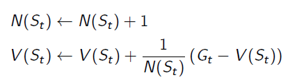
To avoid storing all returns or the sum of returns for all episodes, we transform the equation a little bit when we calculate the new State-Value function:
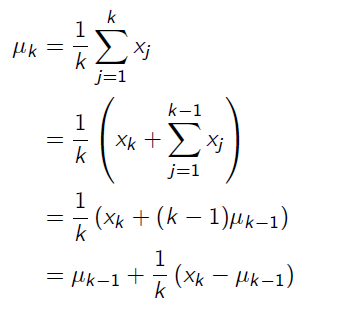
And we get the equation for updating State-Value function:
2. Every-Visit Monte Carlo Evaluation Algorithm
Initialize:
a. π is the policy that needs to be evaluated;
b. V(St) is an arbitary State-Value function;
c. Counter matrix N(St), to record the appearance time of each state;
Repeat in loops:
a. Generate an episode from π
b. For each state s appearing in the episode for every time, calculate new State-Value function V(St)
Population vs. Sample
A online video from MIT(Here we go) reminds me the idea of Population and Sample from Statistics. Population is quite like the whole knowledge on Model-Based learning, but getting samples is easier and more realistic in real life. Monte Carlo is similar to using the distribution of samples to do inference of the population.