Chapter 5 Monte Carlo Methods

不像以前章节，这里不假设有complete knowledge of the environment。

不需要完美的model，只要有experiences就行，用episodes表示，一个episode就是一个完整的从开始到结束的state、action、reward序列。蒙特卡洛方法的特点就是要使用整个序列，举例来说就是必须在一个episode结束后得到了整个序列才能使用蒙特卡洛方法。
蒙特卡洛方法因此可以episode-by-episode的增加，但不是step-by-step的（在线）的增加。
蒙特卡洛方法在这里用于基于averaging complete returns。而且要处理的问题也是nonstationarity

5.1 Monte Carlo Prediction

首先考虑蒙特卡洛方法用于在给定policy下学习state-value function。跟Policy Evaluation(Prediction)类似的情况。原理是大数定理，这也是所有蒙特卡洛方法的基础

First-Visit Monte-Carlo Policy Evaluation：estimate as the average of the returns following first visits to s.
- To evaluate state s
- The fi rst time-step t that state s is visited in an episode,
- Increment counter $N(s) \leftarrow N(s)+1$
- Increment total return $S(s) \leftarrow S(s)+G_t$
- Value is estimated by mean return $V(s)=S(s)/N(s)$
- By law of large numbers, $V(s) \rightarrow v_{\pi}(s) \ \text{as}\ N(s) \rightarrow \infty$
Every-Visit Monte-Carlo Policy Evaluation：estimate as the average of the returns following every visits to s.
- To evaluate state s
- Every time-step t that state s is visited in an episode,
- Increment counter $N(s) \leftarrow N(s)+1$
- Increment total return $S(s) \leftarrow S(s)+G_t$
- Value is estimated by mean return $V(s)=S(s)/N(s)$
- Again, $V(s) \rightarrow v_{\pi}(s) \ \text{as}\ N(s) \rightarrow \infty$

这里的说的对s的visit 是指在一个episode中 state s 出现一次

First-visit MC prediction
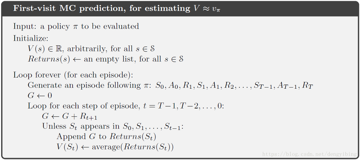
first-visit MC和every-visit MC都收敛到 $v_{\pi}(s)$ ，当visit的数量增加到无限的时候

5.3 Monte Carlo Control

π (s) ≐ \underset{a}{a r g max} q (s, a) .

$\pi(s) \doteq \underset{a}{arg\max} q(s,a).$
policy improvement theorem应用到

π_{k}

$\pi_k$ 和

π_{k + 1}

$\pi_{k+1}$

\begin{aligned} q_{π_{k}} (s, π_{k + 1} (s)) & = q_{π_{k}} (s, \underset{a}{a r g max} q_{π_{k}} (s, a)) \\ = max_{a} q_{π_{k}} (s, a) \\ \geq q_{π_{k}} (s, π_{k} (s)) \\ \geq v_{π_{k}} (s) . \end{aligned}

$\begin{align*} q_{\pi_k}(s,\pi_{k+1}(s)) & = q_{\pi_k}(s,\underset{a}{arg\max} q_{\pi_k}(s,a))\\ & = \underset{a}{\max} q_{\pi_k}(s,a)\\ & \geq q_{\pi_k}(s,\pi_k(s))\\ & \geq v_{\pi_k}(s). \end{align*}$
Monte Carlo ES

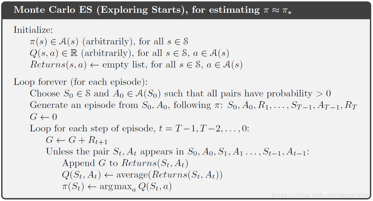
exploring starts就是开始的时候手动给一个好的值

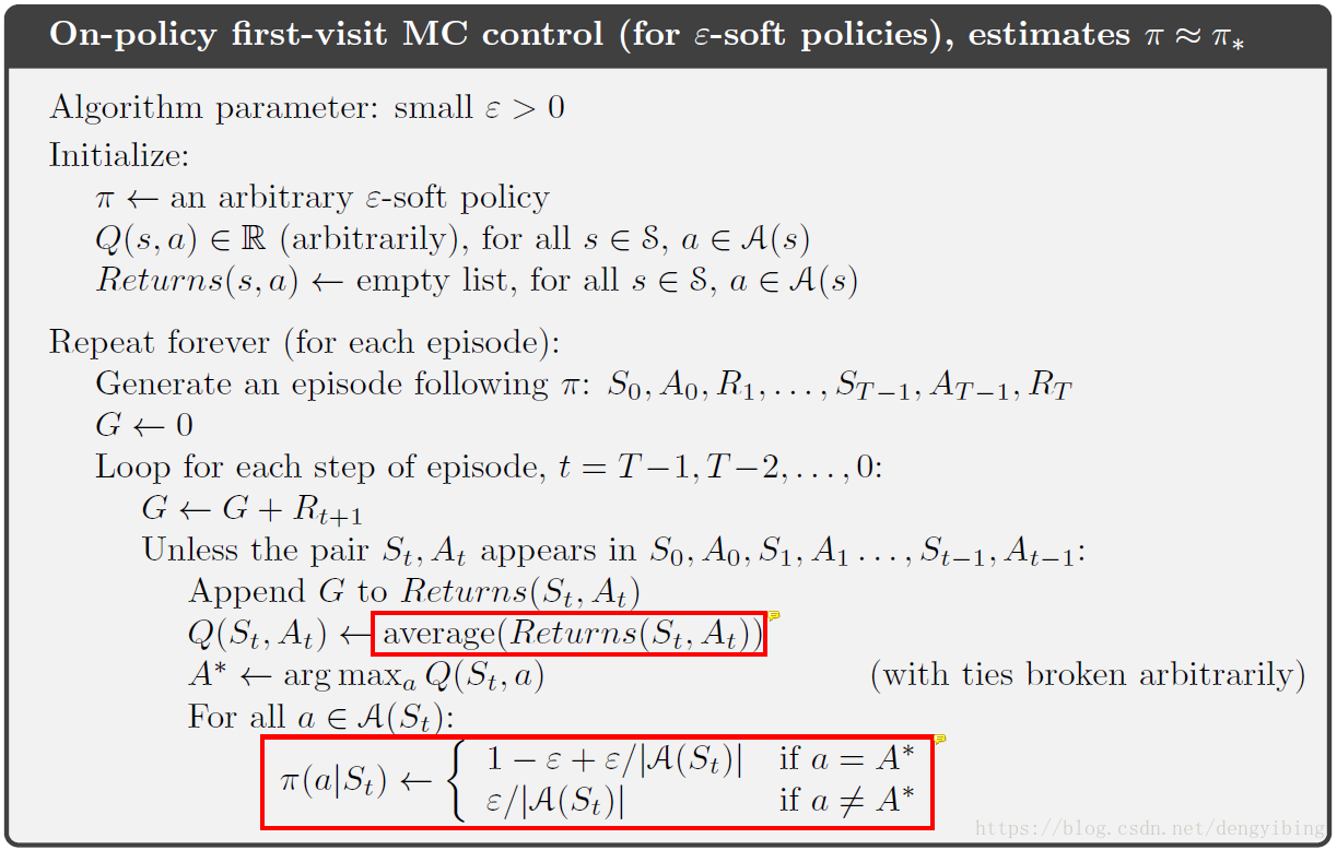
5.4 Monte Carlo Control without Exploring Starts

有两种方法可以避开exploring starts的需求

On-policy learning
- ”Learn on the job”
- Learn about policy $\pi$ from experience sampled from $\pi$
- On-policy更新的policy与产生样本的policy是一样的
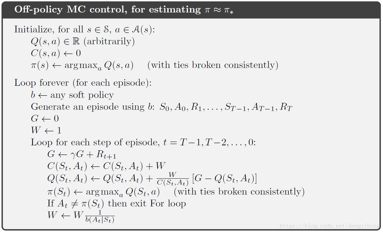
Off-policy learning
- ”Look over someone’s shoulder”
- Learning about policy $\pi$ from experience sampled from $\mu$
- Off-policy更新的policy与产生样本的policy不一样

关于On-policy和Off-policy的定义和关系是后面近似方法的核心

On-policy rst-visit MC control

5.5 Off-policy Prediction via Importance Sampling

off-policy的方差更大，收敛的更慢

on-policy approach实际上是一种妥协，是探索近似最优policy。
off-policy approach使用一种更直观的方式是使用两个policy，一个用来学习并成为the optimal policy，另一个更exploratory，用来generate behavior。

用来学习的policy称为target policy，这里是 $\pi$ ；用来生成行为的policy称为behavior policy，这里是 $b$ 。
In this case we say that learning is from data “off” the target policy, and the overall process is termed off-policy learning.

因为behavior policy更stochastic and more exploratory，所以可以是 $\varepsilon\text{-greedy}$ 方法

Almost all off-policy methods utilize importance sampling, a general technique for estimating expected values under one distribution given samples from another.
We apply importance sampling to off-policy learning by weighting returns according to the relative probability of their trajectories occurring under the target and behavior policies, called the importance-sampling ratio.

给定开始状态 $S_t$ ，后续state-action trajectory在任意policy $\pi$ 下发生的概率

\begin{aligned} P r & {A_{t}, S_{t + 1}, A_{T = 1}, \dots, S_{T} | S_{t}, A_{t : T - 1} \sim π} \\ = π (A_{t} | S_{t}) p (S_{t + 1} | S_{t}, A_{t}) π (A_{t + 1} | S_{t + 1}) \dots p (S_{T} | S_{T - 1}, A_{T - 1}) \\ = \prod_{k = t}^{T - 1} π (A_{k} | S_{k}) p (S_{k + 1} | S_{k}, A_{k}), \end{aligned}

$\begin{align*} Pr & \{ A_t,S_{t+1},A_{T=1},\cdots,S_T|S_t,A_{t:T-1} \sim \pi \} \\ & = \pi(A_t|S_t)p(S_{t+1}|S_t,A_t)\pi(A_{t+1}|S_{t+1})\cdots p({S_T|S_{T-1},A_{T-1}})\\ & = \prod_{k=t}^{T-1} \pi(A_k|S_k)p(S_{k+1}|S_k,A_k), \end{align*}$

注意trajectory，后面蒙特卡洛搜索树会用到这个概念

那么importance sampling ratio为

ρ_{t : T - 1} ≐ \frac{\prod_{k = t}^{T - 1} π (A_{k} | S_{k}) p (S_{k + 1} | S_{k}, A_{k})}{\prod_{k = t}^{T - 1} b (A_{k} | S_{k}) p (S_{k + 1} | S_{k}, A_{k})} = \prod_{k = t}^{T - 1} \frac{π (A_{k} | S_{k})}{b (A_{k} | S_{k})}

$\rho_{t:T-1} \doteq \frac{\prod_{k=t}^{T-1} \pi(A_k|S_k)p(S_{k+1}|S_k,A_k)}{\prod_{k=t}^{T-1} b(A_k|S_k)p(S_{k+1}|S_k,A_k)}=\prod_{k=t}^{T-1} \frac{\pi(A_k|S_k)}{b(A_k|S_k)}$

应用importance ratio。在只有有behavior policy得到的returns $G_t$ 的情况下，想得到在target policy下的expected returns(values)。

E [ρ_{t : T - 1} G_{t} | S_{t} = s] = v_{π} (s)

$\mathbb{E}[\rho_{t:T-1}G_t|S_t=s]=v_{\pi}(s)$

In particular, we can define the set of all time steps in which state s is visited, denoted $J(s)$ . This is for an every-visit method; for a fi rst-visit method, $J(s)$ would only include time steps that were fi rst-visits to s within their episodes.

Ordinary importance sampling:

V (s) ≐ \frac{\sum_{t \in J (s)} ρ_{t : T - 1} G_{t}}{| J (s) |}

$V(s) \doteq \frac{\sum_{t \in J(s)}\rho_{t:T-1}G_t}{|J(s)|}$

Weighted importance sampling:

V (s) ≐ \frac{\sum_{t \in J (s)} ρ_{t : T - 1} G_{t}}{\sum_{t \in J (s)} ρ_{t : T - 1}}

$V(s) \doteq \frac{\sum_{t \in J(s)}\rho_{t:T-1}G_t}{\sum_{t \in J(s)}\rho_{t:T-1}}$

5.6 Incremental Implementation

$W_t=\rho_{t:T-1}$
则有
$V(s) \doteq \frac{\sum_{t=1}^{n-1}W_kG_t}{\sum_{t=1}^{n-1}W_k}, \qquad n \geq 2$

把上面的权重更新写成递增实现
$V_{n+1} \doteq V_n + \frac{W_n}{C_n}[C_n-V_n], \qquad n \geq 1$
和
$G_{n+1} \doteq C_n+W_{n+1}$

Off-policy MC prediction
这里其实就是上面增量的实现weighted importance-sampling。这里只表现了增量实现与importance-sampling的关系

5.7 Off-policy Monte Carlo Control

Off-policy MC control

5.8 *Discounting-aware Importance Sampling

把returns的内部结构添加到discounted rewards的总和的考虑中。这可以减小方差

The essence of the idea is to think of discounting as determining a probability of termination or, equivalently, a degree of partial termination.

$\bar{G}_{t:h} \doteq R_{t+1}+R_{t+2}+\cdots+R_{h}, \qquad 0\leq t \lt h \leq T,$

The conventional full return $G_t$ can be viewed as a sum of at partial returns

\begin{aligned} G_{t} & ≐ R_{t + 1} + γ R_{t + 2} + γ^{2} R_{t + 3} + \dots + γ^{T - t - 1} R_{T} \\ = (1 - γ) R_{t + 1} \\ + (1 - γ) γ (R_{t + 1} + R_{t + 2}) \\ + (1 - γ) γ^{2} (R_{t + 1} + R_{t + 2} + R_{t + 3}) \\ ⋮ \\ + (1 - γ) γ^{T - t - 2} (R_{t + 1} + R_{t + 2} + \dots + R_{T - 1}) \\ + γ^{T - t - 1} (R_{t + 1} + R_{t + 2} + \dots + R_{T - 1}) \\ = (1 - γ) \sum_{h = t + 1}^{T - 1} γ^{h - t - 1} {\bar{G}}_{t : h} + γ^{T - t - 1} {\bar{G}}_{t : T} \end{aligned}

$\begin{align*} G_t & \doteq R_{t+1}+\gamma R_{t+2}+\gamma^2 R_{t+3}+\cdots+\gamma^{T-t-1}R_T\\ &= (1-\gamma)R_{t+1}\\ & + (1-\gamma)\gamma (R_{t+1}+R_{t+2})\\ & + (1-\gamma)\gamma^2 (R_{t+1}+R_{t+2}+R_{t+3})\\ \vdots\\ & + (1-\gamma)\gamma^{T-t-2} (R_{t+1}+R_{t+2}+\cdots+R_{T-1})\\ & + \gamma^{T-t-1}(R_{t+1}+R_{t+2}+\cdots+R_{T-1})\\ & = (1-\gamma)\sum_{h=t+1}^{T-1} \gamma^{h-t-1} \bar{G}_{t:h} + \gamma^{T-t-1}\bar{G}_{t:T} \end{align*}$
则有
ordinary importance-sampling estimator

V (s) ≐ \frac{\sum_{t \in J (s)} ((1 - γ) \sum_{h = t + 1}^{T (t) - 1} γ^{h - t - 1} ρ_{t : h - 1} {\bar{G}}_{t : h} + γ^{T (t) - t - 1} ρ_{t : T (t) - 1} {\bar{G}}_{t : T (t)})}{| J (s) |}

$V(s) \doteq \frac {\sum_{t \in J(s)}((1-\gamma)\sum_{h=t+1}^{T(t)-1}\gamma^{h-t-1}\rho_{t:h-1}\bar{G}_{t:h}+\gamma^{T(t)-t-1}\rho_{t:T(t)-1}\bar{G}_{t:T(t)})} {|J(s)|}$

weighted importance-sampling estimator

V (s) ≐ \frac{\sum_{t \in J (s)} ((1 - γ) \sum_{h = t + 1}^{T (t) - 1} γ^{h - t - 1} ρ_{t : h - 1} {\bar{G}}_{t : h} + γ^{T (t) - t - 1} ρ_{t : T (t) - 1} {\bar{G}}_{t : T (t)})}{\sum_{t \in J (s)} ((1 - γ) \sum_{h = t + 1}^{T (t) - 1} γ^{h - t - 1} ρ_{t : h - 1} + γ^{T (t) - t - 1} ρ_{t : T (t) - 1})}

$V(s) \doteq \frac {\sum_{t \in J(s)}((1-\gamma)\sum_{h=t+1}^{T(t)-1}\gamma^{h-t-1}\rho_{t:h-1}\bar{G}_{t:h}+\gamma^{T(t)-t-1}\rho_{t:T(t)-1}\bar{G}_{t:T(t)})} {\sum_{t \in J(s)}((1-\gamma)\sum_{h=t+1}^{T(t)-1}\gamma^{h-t-1}\rho_{t:h-1}+\gamma^{T(t)-t-1}\rho_{t:T(t)-1})}$

5.9 *Per-decision Importance Sampling

另外一种把structure of the return作为rewards的总和，可以被考虑在off-policy importance sampling中。也可以减小方差

\begin{aligned} ρ_{t : T - 1} G_{t} & = ρ_{t : T - 1} (R_{t + 1} + γ R_{t + 2} + \dots + γ^{T - t - 1} R_{T}) \\ = ρ_{t : T - 1} R_{t + 1} + γ ρ_{t : T - 1} R_{t + 2} + \dots + γ^{T - t - 1} ρ_{t : T - 1} R_{T}) \end{aligned}

$\begin{align*} \rho_{t:T-1}G_t & = \rho_{t:T-1}(R_{t+1}+\gamma R_{t+2}+\cdots+\gamma^{T-t-1}R_T)\\ & = \rho_{t:T-1}R_{t+1}+\gamma \rho_{t:T-1}R_{t+2}+\cdots+\gamma^{T-t-1}\rho_{t:T-1}R_T) \end{align*}$
上式的第一个子项可以写为

ρ_{t : T - 1} R_{t + 1} = \frac{π (A_{t} | S_{t})}{b (A_{t} | S_{t})} \frac{π (A_{t + 1} | S_{t + 1})}{b (A_{t + 1} | S_{t + 1})} \frac{π (A_{t + 2} | S_{t + 2})}{b (A_{t + 2} | S_{t + 2})} \dots \frac{π (A_{T - 1} | S_{T - 1})}{b (A_{T - 1} | S_{T - 1})} R_{t + 1}

$\rho_{t:T-1}R_{t+1} = \frac{\pi(A_t|S_t)}{b(A_t|S_t)} \frac{\pi(A_{t+1}|S_{t+1})}{b(A_{t+1}|S_{t+1})} \frac{\pi(A_{t+2}|S_{t+2})}{b(A_{t+2}|S_{t+2})} \cdots \frac{\pi(A_{T-1}|S_{T-1})}{b(A_{T-1}|S_{T-1})} R_{t+1}$

注意到上式中的各项，只有第一项和最后一项(the reward)是相关的；其他各项都是独立随机变量，它们的期望值为1

E [\frac{π (A_{k} | S_{k})}{b (A_{k} | S_{k})}] ≐ \sum_{a} b (a | S_{k}) \frac{π (a | S_{k})}{b (a | S_{k})} = \sum_{a} π (a | S_{k}) = 1

$\mathbb{E}[\frac{\pi(A_k|S_k)}{b(A_k|S_k)}] \doteq \sum_a b(a|S_k)\frac{\pi(a|S_k)}{b(a|S_k)} = \sum_a \pi(a|S_k) = 1$

所有的比率值中，只有第一项留下来了，则有

E [ρ_{t : T - 1} R_{t + 1}] = [ρ_{t : t} R_{t + 1}]

$\mathbb{E}[\rho_{t:T-1}R_{t+1}]=\mathbb[\rho_{t:t}R_{t+1}]$

重复上述分析过程则可以得到

E [ρ_{t : T - 1} G_{t}] = E [{\bar{G}}_{t}]

$\mathbb{E}[\rho_{t:T-1}G_t]=\mathbb{E}[\bar G_t]$

其中

{\bar{G}}_{t} = ρ_{t : t} R_{t + 1} + γ ρ_{t : t + 1} R_{t + 2} + γ^{2} ρ_{t : t + 2} R_{t + 3} + \dots + γ^{T - t - 1} ρ_{t : T - 1} R_{T}

$\bar G_t = \rho_{t:t}R_{t+1}+\gamma \rho_{t:t+1}R_{t+2}+\gamma^2 \rho_{t:t+2}R_{t+3}+\cdots+\gamma^{T-t-1} \rho_{t:T-1}R_T$
我们称这个想法为 per-decision importance sampling

使用 $\bar G_t$ 的ordinary-importance-sampling estimator

V (s) ≐ \frac{\sum_{t \in J (s)} {\bar{G}}_{t}}{| J (s) |}

$V(s) \doteq \frac{\sum_{t \in J(s)}\bar G_t}{|J(s)|}$