牛顿法求解非线性方程组(Octave)

Octave:5.1.0
参考书籍：OctaveAtBFH.pdf（自行网上搜索）

需要两个文件：

函数文件fsolveNewton.m，函数名和文件名一定要对应
脚本文件nonlinear_test.m

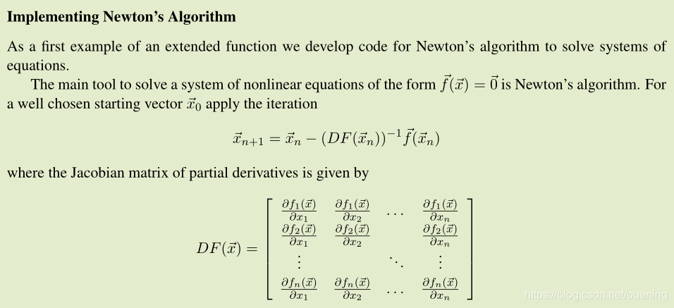
参考书籍OctaveAtBFH第72页内容：
在这里插入图片描述

`fsolveNewton.m` 程序

function [x, iter, fval] = fsolveNewton(f ,x0 , tolx , dfdx)
  % [x, iter ] = fsolveNewton(f ,x0 , tolx , dfdx)
  % use Newtons method to solve a system of equations f (x)=0,
  % the number of equations and unknowns have to match
  % the Jacobian matrix is either given by the function dfdx or
  % determined with finite difference computations
  %
  % input parameters :
  % f string with the function name
  % function has to return a column vector
  % x0 starting value
  % tolx allowed tolerances ,
  % a vector with the maximal tolerance for each component
  % if tolx is a scalar , use this value for each of the components
  % dfdx string with function name to compute the Jacobian
  %
  % output parameters :
  % x vector with the approximate solution
  % iter number of required iterations
  % it iter >20 then the algorithm did not converge
  if (( nargin < 3)|( nargin >=5)) % 要求输出的参数为3个或4个，dxfx为缺省参数
  usage( 'wrong number of arguments in fsolveNewton(f ,x0 , tolx , dfdx ) ');
  end
  maxit = 20; % maximal number of iterations
  x = x0;
  iter = 0;
  if isscalar ( tolx ) % 如果容差是一个标量，需要将其转化为维度和未知数维度一致，比如有n个未知数，该容差会应用到这n个解中
    tolx = tolx*ones( size (x0 )); 
  end
  dx = 100*abs( tolx ); % 计算步长，容差的100倍，比如容差设置为1e-6时，dx为1e-4，当然需要考虑向量形式
  f0 = feval (f ,x);    % 获得初值
  m = length (f0);     
  n = length (x);       % n维列向量
  if (n ~= m) % 这里需要满足满秩要求，即含n个未知数的方程组要有同样n个方程才能求解
    error ('number of equations not equal number of unknown')
  end
  if (n ~= length (dx))
     error ('tolerance not correctly specified' )
  end
  jac = zeros (m,n); % 如果非线性方程组有m个方程，每个方程含未知数为n个，那么其雅可比矩阵大小为（m，n）reserve memory for the Jacobian
  done = false ; % Matlab has no ’do until ’
  
  while ~done
    if nargin==4 % 如果输入4个参数，那么会使用提供的雅克比矩阵
      jac = feval (dfdx ,x);
    else % use a finite difference approx for Jacobian，如果没有提供，使用有限差分的方法逼近
      dx = dx/100; % 这里dx步长缩小100倍，记住这里dx是一个n维列向量
##      disp(dx);
      for jj= 1:n
        xn = x;   % x
        xn( jj ) = xn(jj) + dx(jj); 
        % 理解为：f'(x)=(f(x+dx)-f(x))/dx，这里f(x)为f0
        jac (: , jj ) = (( feval (f ,xn)-f0 )/dx( jj )); 
        disp(jac); % 输出查看jac矩阵
        printf('\n')
      end
    end
    % jac矩阵是随着每次迭代而不断更新，类比单变量的牛顿法，每次迭代都要计算变量在该次迭代的一阶导数，供下一次迭代计算
    % 注意左除符号，jac是(n,n)大小的矩阵，f0是(n,1)大小的向量，同时该结果赋值给dx，起到了变步长的作用，越接近解时步长越小，步长dx随jac\f0变化
    dx = jac\f0 ; % 可以看出jac又是关于dx的函数，加速迭代
    x = x - dx;
    
    % 下面方式是固定步长方式（同时需要注释掉前面代码：dx=dx/100），jac矩阵更新过程中不利于已有信息进行更新
##    tmp = jac\f0;
##    disp(tmp);
##    x = x-tmp;
    iter = iter +1;
    f0 = feval (f ,x);  % 重新赋值f0
    if (( iter >=maxit )|( abs(dx)<tolx ))
      done = true ;
  end
  fval = feval(f,x);
end

脚本文件`nonlinear_test.m`

clear *
clc;
x0 = [1;1]; % choose the starting value
function y = f (x) % define the system of equations
y = [x(1)**2 + 4*x(2)**2 - 1;
      4*x(1)**4 + x(2)**2 - 1];
endfunction
function y = dfdx(x) % Jacobian
y = [2*x(1) , 8*x(2);
      16*x(1)**3 , 2*x(2)**2];
endfunction
##[x, iter, fval] = fsolveNewton('f' ,x0,1e-4*[1;1]) % use a finite difference Jacobian
[x, iter, fval] = fsolveNewton('f' ,x0,1e-6)   % higher accuracy
##[x, iter, fval] = fsolveNewton('f' ,x0,1e-6,'dfdx') % user provided Jacobian
% Octave自带函数fsolve求解
[x, fval, info] = fsolve(@f,x0)

运行结果

    2.00000    0.00000
   16.00002    0.00000

    2.0000    8.0000
   16.0000    2.0000

   1.6148   8.0000
   8.4221   2.0000

   1.6148   4.4052
   8.4221   1.1013

   1.4195   4.4052
   5.7205   1.1013

   1.41950   3.12885
   5.72047   0.78221

   1.36790   3.12885
   5.11914   0.78221

   1.36790   2.92834
   5.11914   0.73208

   1.36442   2.92834
   5.08011   0.73208

   1.36442   2.92468
   5.08011   0.73117

   1.36439   2.92468
   5.07977   0.73117

   1.36439   2.92468
   5.07977   0.73117

x =

   0.68219
   0.36559

iter =  6
fval =

   0.0000e+00
   2.2204e-16

x =

   0.68219
   0.36559

fval =

   0.000000000039742
   0.000000000330773

info =  1

关键点

（1）步长更新利用了雅可比矩阵的信息，加速了迭代运算，而不是常规的固定步长，经测试，修改为固定步长的情况下，保证精度一定时，求解上述问题需要的迭代次数为20，而利用了雅可比矩阵加速迭代只用了6次迭代；

（2）我们知道单变量非线性方程求根的基本牛顿迭代公式为： $x_{n+1}=x_n-\frac{f(x_n)}{f'(x_n)}$
迭代过程中关键是计算 $f'(x_n)$ ，在 $f(x)$ 给定的情况下，如果 $f'(x)$ 没有事先给定，那么就根据从导数的定义出发：
$f^{\prime}\left(x_{0}\right)=\lim _{\Delta x \rightarrow 0} \frac{\Delta y}{\Delta x}=\lim _{\Delta x \rightarrow 0} \frac{f\left(x_{0}+\Delta x\right)-f\left(x_{0}\right)}{\Delta x}$
我们取一个很小的步长 $\Delta x=h$ 来计算导数的近似值。

多元函数的迭代公式为：
$\vec{x}_{n+1}=\vec{x}_{n}-\left(\nabla F\left(\vec{x}_{n}\right)\right)^{-1} \vec{f}\left(\vec{x}_{n}\right)$

式中 $x \in \mathbb{R}^n$ ， $\nabla F(\bar{x_{n}})$ 得到雅可比矩阵，写成分量形式为（省略向量标记）： $\nabla F({x_{n}})=\frac{\partial F_i(x_n)}{\partial x_j},\quad i,j=1,2,\cdots n$ 是 $n \times n$ 大小的矩阵，因此从公式中矩阵的逆乘上函数值，写成代码形式就是x = x - jac\f0，关于左乘和右乘问题这里就不详细叙述了。