这次主要做的是基于sift特征匹配然后使用RANSAC全景图像拼接
下面简单地对RANSAC算法进行介绍,参考自:https://blog.csdn.net/robinhjwy/article/details/79174914
一、RANSAC概述
RANSAC算法的输入是一组观测数据,一个可以解释或者适应于观测数据的参数化模型,一些可信的参数。
RANSAC通过反复选择数据中的一组随机子集来达成目标。被选取的子集被假设为局内点,并用下述方法进行验证:
1.首先我们先随机假设一小组局内点为初始值。然后用此局内点拟合一个模型,此模型适应于假设的局内点,所有的未知参数都能从假设的局内点计算得出。
2.用1中得到的模型去测试所有的其它数据,如果某个点适用于估计的模型,认为它也是局内点,将局内点扩充。
3.如果有足够多的点被归类为假设的局内点,那么估计的模型就足够合理。
4.然后,用所有假设的局内点去重新估计模型,因为此模型仅仅是在初始的假设的局内点估计的,后续有扩充后,需要更新。
5.最后,通过估计局内点与模型的错误率来评估模型。
整个这个过程为迭代一次,此过程被重复执行固定的次数,每次产生的模型有两个结局:
1、要么因为局内点太少,还不如上一次的模型,而被舍弃,
2、要么因为比现有的模型更好而被选用。
二、RANSAC示例
一个简单的例子是从一组观测数据中找出合适的2维直线。假设观测数据中包含局内点和局外点,其中局内点近似的被直线所通过,而局外点远离于直线。简单的最小二乘法不能找到适应于局内点的直线,原因是最小二乘法尽量去适应包括局外点在内的所有点。相反,RANSAC能得出一个仅仅用局内点计算出模型,并且概率还足够高。但是,RANSAC并不能保证结果一定正确,为了保证算法有足够高的合理概率,我们必须小心的选择算法的参数。

三、RANSAC原理
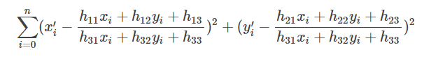
OpenCV中滤除误匹配对采用RANSAC算法寻找一个最佳单应性矩阵H,矩阵大小为3×3。RANSAC目的是找到最优的参数矩阵使得满足该矩阵的数据点个数最多,通常令h33=1h33=1来归一化矩阵。由于单应性矩阵有8个未知参数,至少需要8个线性方程求解,对应到点位置信息上,一组点对可以列出两个方程,则至少包含4组匹配点对。

其中(x,y)表示目标图像角点位置,(x’,y’)为场景图像角点位置,s为尺度参数。
RANSAC算法从匹配数据集中随机抽出4个样本并保证这4个样本之间不共线,计算出单应性矩阵,然后利用这个模型测试所有数据,并计算满足这个模型数据点的个数与投影误差(即代价函数),若此模型为最优模型,则对应的代价函数最小。
RANSAC算法步骤:
1. 随机从数据集中随机抽出4个样本数据 (此4个样本之间不能共线),计算出变换矩阵H,记为模型M;
2. 计算数据集中所有数据与模型M的投影误差,若误差小于阈值,加入内点集 I ;
3. 如果当前内点集 I 元素个数大于最优内点集 I_best , 则更新 I_best = I,同时更新迭代次数k ;
4. 如果迭代次数大于k,则退出 ; 否则迭代次数加1,并重复上述步骤;
注:迭代次数k在不大于最大迭代次数的情况下,是在不断更新而不是固定的,见上方k的更新;
其中,p为置信度,一般取0.995;w为”内点”的比例 ; m为计算模型所需要的最少样本数=4;
求得单应矩阵后就好办了,把内点留下,内点就是筛选后的好用的点,外点舍弃,外点就有可能是误匹配的点。
四、RANSAC的优点和缺点
RANSAC的优点是它能鲁棒的估计模型参数。例如,它能从包含大量局外点的数据集中估计出高精度的参数。RANSAC的缺点是它计算参数的迭代次数没有上限;如果设置迭代次数的上限,得到的结果可能不是最优的结果,甚至可能得到错误的结果。RANSAC只有一定的概率得到可信的模型,概率与迭代次数成正比。RANSAC的另一个缺点是它要求设置跟问题相关的阀值。
RANSAC只能从特定的数据集中估计出一个模型,如果存在两个(或多个)模型,RANSAC不能找到别的模型。
本次实验主要使用的是sift特征匹配和RANSAC算法,关于sift特征匹配在我的上一篇特征点提取和匹配相关的文章中有对sift特征匹配的详尽介绍此处就不再多做说明。
下面是这次实验的主函数代码:
from pylab import *
from numpy import *
from PIL import Image

# If you have PCV installed, these imports should work
from PCV.geometry import homography, warp
from PCV.localdescriptors import sift


# 设置数据文件夹的路径
featname = ['D:\pythonxy\image\we'+str(i+1)+'.sift' for i in range(5)]
imname = ['D:\pythonxy\image\we'+str(i+1)+'.jpg' for i in range(5)]

# 使用sift特征自动找到匹配对应
l = {}
d = {}
for i in range(5):
    sift.process_image(imname[i],featname[i])
    l[i],d[i] = sift.read_features_from_file(featname[i])

matches = {}
for i in range(4):
    matches[i] = sift.match(d[i+1],d[i])

# 可视化两张图像
for i in range(4):
    im1 = array(Image.open(imname[i]))
    im2 = array(Image.open(imname[i+1]))
    figure()
    sift.plot_matches(im2,im1,l[i+1],l[i],matches[i],show_below=True)


# 将匹配项转化为特征点
def convert_points(j):
    ndx = matches[j].nonzero()[0]
    fp = homography.make_homog(l[j+1][ndx,:2].T)
    ndx2 = [int(matches[j][i]) for i in ndx]
    tp = homography.make_homog(l[j][ndx2,:2].T)

    # switch x and y - TODO this should move elsewhere
    fp = vstack([fp[1],fp[0],fp[2]])
    tp = vstack([tp[1],tp[0],tp[2]])
    return fp,tp


# 估计单应性矩阵
model = homography.RansacModel()

fp,tp = convert_points(1)
H_12 = homography.H_from_ransac(fp,tp,model)[0] #im 1 to 2

fp,tp = convert_points(0)
H_01 = homography.H_from_ransac(fp,tp,model)[0] #im 0 to 1

tp,fp = convert_points(2) #NB: reverse order
H_32 = homography.H_from_ransac(fp,tp,model)[0] #im 3 to 2

tp,fp = convert_points(3) #NB: reverse order
H_43 = homography.H_from_ransac(fp,tp,model)[0] #im 4 to 3


# 扭曲图像
delta = 2000 # for padding and translation

im1 = array(Image.open(imname[1]), "uint8")
im2 = array(Image.open(imname[2]), "uint8")
im_12 = warp.panorama(H_12,im1,im2,delta,delta)

im1 = array(Image.open(imname[0]), "f")
im_02 = warp.panorama(dot(H_12,H_01),im1,im_12,delta,delta)

im1 = array(Image.open(imname[3]), "f")
im_32 = warp.panorama(H_32,im1,im_02,delta,delta)

im1 = array(Image.open(imname[4]), "f")
im_42 = warp.panorama(dot(H_32,H_43),im1,im_32,delta,2*delta)


figure()
imshow(array(im_42, "uint8"))
axis('off')
show()
其中使用sift特征自动找到匹配对应使用到了sift.py文件里的process_image和read_features_from_file和match方法
sift.process_image方法的作用是处理一幅图像,然后将特征结果保存在文件中,代码如下:
def process_image(imagename,resultname,params="--edge-thresh 10 --peak-thresh 5"):
    """ process an image and save the results in a file"""
    path = os.path.abspath(os.path.join(os.path.dirname("__file__"),os.path.pardir))
    path = path+"\\utils\\win32vlfeat\\sift.exe "
    if imagename[-3:] != 'pgm':
	    #create a pgm file
		 im = Image.open(imagename).convert('L')
		 im.save('tmp.pgm')
		 imagename = 'tmp.pgm'
    cmmd = str("D:\pythonxy\win64vlfeat\sift.exe "+imagename+" --output="+resultname+
				" "+params)
    os.system(cmmd)
    print 'processed', imagename, 'to', resultname
sift.read_features_from_file方法的作用是读取图像的特征属性值,然后将其以矩阵的形式返回,代码如下:
def read_features_from_file(filename):
	""" read feature properties and return in matrix form"""
	f = loadtxt(filename)
	return f[:,:4],f[:,4:] # feature locations, descriptors
sift.match方法的作用是对于第一幅图像中的每个描述子,选取其在第二幅图像中的匹配,代码如下:
def match(desc1,desc2):
	""" for each descriptor in the first image,
		select its match in the second image.
		input: desc1 (descriptors for the first image),
		desc2 (same for second image). """

	desc1 = array([d/linalg.norm(d) for d in desc1])
	desc2 = array([d/linalg.norm(d) for d in desc2])

	dist_ratio = 0.6
	desc1_size = desc1.shape

	matchscores = zeros((desc1_size[0],1))
	desc2t = desc2.T #precompute matrix transpose
	for i in range(desc1_size[0]):
		dotprods = dot(desc1[i,:],desc2t) #vector of dot products
		dotprods = 0.9999*dotprods
		#inverse cosine and sort, return index for features in second image
		indx = argsort(arccos(dotprods))

		#check if nearest neighbor has angle less than dist_ratio times 2nd
		if arccos(dotprods)[indx[0]] < dist_ratio * arccos(dotprods)[indx[1]]:
			matchscores[i] = int(indx[0])

	return matchscores
读取特征后,通过在图像上绘制出他们的位置,可以将其可视化,这个功能使用到了sift.py中plot_matches方法,此方法的作用是显示一副带有连接匹配之间连线的图片,代码如下:
def plot_matches(im1,im2,locs1,locs2,matchscores,show_below=True):
	""" show a figure with lines joining the accepted matches
		input: im1,im2 (images as arrays), locs1,locs2 (location of features),
		matchscores (as output from 'match'), show_below (if images should be shown below). """

	im3 = appendimages(im1,im2)
	if show_below:
		im3 = vstack((im3,im3))

	# show image
	imshow(im3)

	# draw lines for matches
	cols1 = im1.shape[1]
	for i in range(len(matchscores)):
		if matchscores[i] > 0:
			plot([locs1[i,0], locs2[int(matchscores[i,0]),0]+cols1], [locs1[i,1], locs2[int(matchscores[i,0]),1]], 'c')
	axis('off')
然后将匹配转换成齐次坐标点的函数,使用了homography.py文件中的make_homog方法,该方法的作用是将一组点(dim*n数组)转换为齐次坐标。代码如下:
def make_homog(points):
    """ Convert a set of points (dim*n array) to
        homogeneous coordinates. """

    return vstack((points,ones((1,points.shape[1]))))
接着就是估计单应性矩阵,使用了homography.py文件中的H_from_ransac方法,H_from_ransac方法的作用是使用RANSAC稳健性估计点对应间的单应性矩阵H,代码如下:
def H_from_ransac(fp,tp,model,maxiter=1000,match_theshold=10):
    """ Robust estimation of homography H from point
        correspondences using RANSAC (ransac.py from
        http://www.scipy.org/Cookbook/RANSAC).

        input: fp,tp (3*n arrays) points in hom. coordinates. """

    from PCV.tools import ransac

    # 对应点组
    data = vstack((fp,tp))

    # 计算H,并返回
    H,ransac_data = ransac.ransac(data.T,model,4,maxiter,match_theshold,10,return_all=True)
    return H,ransac_data['inliers']
该方法允许提供阈值和最小期望的点对数目。最重要的参数是最大迭代次数:程序退出太早可能得到一个坏解;迭代次数太多会占用太多时间。方法返回的结果为单应性矩阵和对应该单应性矩阵的正确点对。
我们还要使用RANSAC算法来求解单应性矩阵,首先需要将下面用于测试单应性矩阵的类的模型类homograpy.py文件中,代码如下:
class RansacModel(object):
    """ Class for testing homography fit with ransac.py from
        http://www.scipy.org/Cookbook/RANSAC"""

    def __init__(self,debug=False):
        self.debug = debug

    def fit(self, data):
        """ Fit homography to four selected correspondences. """

        # transpose to fit H_from_points()
        data = data.T

        # from points
        fp = data[:3,:4]
        # target points
        tp = data[3:,:4]

        # fit homography and return
        return H_from_points(fp,tp)

    def get_error( self, data, H):
        """ Apply homography to all correspondences,
            return error for each transformed point. """

        data = data.T

        # from points
        fp = data[:3]
        # target points
        tp = data[3:]

        # transform fp
        fp_transformed = dot(H,fp)

        # normalize hom. coordinates
        fp_transformed = normalize(fp_transformed)

        # return error per point
        return sqrt( sum((tp-fp_transformed)**2,axis=0) )
这个类中包含fit()方法。该方法仅仅接受由ransac选择的4个对应点对,然后拟合一个单应性矩阵。4个点对是计算单应性矩阵所需的最小数目。由于get_error方法都每个对应点对使用该单应性矩阵然后返回相应的平方距离之和,因此RANSAC算法能够判断哪些点对是正确的,哪些是错误的。
估计出图像间的单应性矩阵之后我们需要将所有的图像扭曲到一个公共的图像平面上。我们将中心图像左边或者右边的区域填充0,以便为扭曲的图像腾出空间。这里使用到了warp.py文件中的panorama方法,该方法的作用是使用单应性矩阵H协调两幅图像,创建水平全景图像。代码如下:
def panorama(H,fromim,toim,padding=2400,delta=2400):
    """ Create horizontal panorama by blending two images
        using a homography H (preferably estimated using RANSAC).
        The result is an image with the same height as toim. 'padding'
        specifies number of fill pixels and 'delta' additional translation. """

    # check if images are grayscale or color
    is_color = len(fromim.shape) == 3

    # homography transformation for geometric_transform()
    def transf(p):
        p2 = dot(H,[p[0],p[1],1])
        return (p2[0]/p2[2],p2[1]/p2[2])

    if H[1,2]<0: # fromim is to the right
        print 'warp - right'
        # transform fromim
        if is_color:
            # pad the destination image with zeros to the right
            toim_t = hstack((toim,zeros((toim.shape[0],padding,3))))
            fromim_t = zeros((toim.shape[0],toim.shape[1]+padding,toim.shape[2]))
            for col in range(3):
                fromim_t[:,:,col] = ndimage.geometric_transform(fromim[:,:,col],
                                        transf,(toim.shape[0],toim.shape[1]+padding))
        else:
            # pad the destination image with zeros to the right
            toim_t = hstack((toim,zeros((toim.shape[0],padding))))
            fromim_t = ndimage.geometric_transform(fromim,transf,
                                    (toim.shape[0],toim.shape[1]+padding))
    else:
        print 'warp - left'
        # add translation to compensate for padding to the left
        H_delta = array([[1,0,0],[0,1,-delta],[0,0,1]])
        H = dot(H,H_delta)
        # transform fromim
        if is_color:
            # pad the destination image with zeros to the left
            toim_t = hstack((zeros((toim.shape[0],padding,3)),toim))
            fromim_t = zeros((toim.shape[0],toim.shape[1]+padding,toim.shape[2]))
            for col in range(3):
                fromim_t[:,:,col] = ndimage.geometric_transform(fromim[:,:,col],
                                            transf,(toim.shape[0],toim.shape[1]+padding))
        else:
            # pad the destination image with zeros to the left
            toim_t = hstack((zeros((toim.shape[0],padding)),toim))
            fromim_t = ndimage.geometric_transform(fromim,
                                    transf,(toim.shape[0],toim.shape[1]+padding))

    # blend and return (put fromim above toim)
    if is_color:
        # all non black pixels
        alpha = ((fromim_t[:,:,0] * fromim_t[:,:,1] * fromim_t[:,:,2] ) > 0)
        for col in range(3):
            toim_t[:,:,col] = fromim_t[:,:,col]*alpha + toim_t[:,:,col]*(1-alpha)
    else:
        alpha = (fromim_t > 0)
        toim_t = fromim_t*alpha + toim_t*(1-alpha)

    return toim_t
下面是本次实验的远景拍摄的结果图:

这是针对于远景图片拼接的结果图,因为将五张图片的像素调为1000*1280,所以放大后看会比较模糊,但是可以大致的看出拼接的结果是不错的,因为拍摄的时候光线位置没有太大的变化所以交接的位置线不会太明显,比较好的还原了拍摄的全景图。
下面是本次实验的有层次拍摄的结果图:

这是针对有层次的图片拼接的结果图,因为拍摄时的光线变化问题拼接的交界线有明暗变化,但是还是比较完整地把原来的景色拼接出来了。
下面是本次实验的近景拍摄的结果图:

这可以算是本次实验我最满意的一张结果图,图片比较清晰并且没有明暗交错,还原程度较高但是对左边的图片进行了太大的拉伸,显得不够自然。