1.原理
- 检测并提取图像的特征和关键点
- 匹配两个图像之间的描述符
- 使用RANSAC算法使用我们匹配的特征向量估计单应矩阵
- 拼接图像
步骤一和步骤二过程是运用SIFT局部描述算子检测图像中的关键点和特征,SIFT特征是基于物体上的一些局部外观的兴趣点而与影像的大小和旋转无关。对于光线、噪声、些微视角改变的容忍度也很高。
而接下来即步骤三是找到重叠的图片部分,连接所有图片之后就可以形成一个基本的全景图了。匹配图片最常用的方式是采用RANSAC(RANdom SAmple Consensus, 随机抽样一致),用此排除掉不符合大部分几何变换的匹配。之后利用这些匹配的点来**“估算单应矩阵” (Homography Estimation),也就是将其中一张图像通过关联性和另一张匹配。
2.SIFT算法
2.1算法特点
与上一期讲到的Harris角点检测不同
1.具有较好的稳定性和不变性,能够适应旋转、尺度缩放、亮度的变化,能在一定程度上不受视角变化、仿射变换、噪声的干扰
2.区分性好,能够在海量特征数据库中进行快速准确的区分信息进行匹配
3.多量性,就算只有单个物体,也能产生大量特征向量
4.高速性,能够快速的进行特征向量匹配
5.可扩展性,能够与其它形式的特征向量进行联合
2.2对比Harris角点检测
原图:

Harris角点检测:
sift特征:

很明显准确性提高了特别多,并且由于图像过大,在进行harris角点检测的时候,用了将近2个小时才完成,而sift只需要几分钟,体现了其高速性,并且能避免干扰,因此图像拼接我们使用sift算法
2.3 SIFT算法能解决的问题
1.目标的旋转、缩放、平移(RST)
2.图像仿射/投影变换(视点viewpoint )
3.弱光照影响( ilumination)
4.部分目标遮挡(occlusion)
5.杂物场景( clutter)
6.噪声
2.4 SIFT算法实现特征匹配的流程
1.建立高斯差分金字塔

2. 提取关键点:关键点是一些十分突出的不会因光照、尺度、旋转等因素而消失的点,比如角点、边缘点、暗区域的亮点以及亮区域的暗点。此步骤是搜索所有尺度空间上的图像位置。通过高斯微分函数来识别潜在的具有尺度和旋转不变的兴趣点。

3.定位关键点并确定特征方向:在每个候选的位置上,通过一个拟合精细的模型来确定位置和尺度。关键点的选择依据于它们的稳定程度。然后基于图像局部的梯度方向,分配给每个关键点位置一个或多个方向。所有后面的对图像数据的操作都相对于关键点的方向、尺度和位置进行变换,从而提供对于这些变换的不变性。

4.通过各关键点的特征向量,进行两两比较找出相互匹配的若干对特征点,建立景物间的对应关系
3 sift特征检测实现
3.1 安装 vlfeat python图像处理工具
VLFeat是一个跨平台的开源机器视觉库,它囊括了当前流行的机器视觉算法,如SIFT, MSER, HOG, 同时还包含了诸如K-MEANS, Hierarchical K-means的聚类算法。这个库的安装有些特殊和其他python官网可以找到的其他库的安装不一样。
1.进入vlfeat库的下载网站 https://www.vlfeat.org/
2.点击下图红框位置下载。


记得一定要安装正确的版本 否则之后会出现错误
  File "C:\Users\95490\Desktop\计算机视觉python\sifttest1.py", line 14, in <module>
    l1, d1 ,d2,d3= sift.read_features_from_file('test.sift')

  File "C:\Users\95490\AppData\Roaming\Python\Python37\site-packages\PCV\localdescriptors\sift.py", line 26, in read_features_from_file
    return f[:,:4],f[:,4:] # feature locations, descriptors

IndexError: too many indices for array: array is 1-dimensional, but 2 were indexed
然后将cmmd中的目录修改为你自己放置的Vlfeat bin所在目录。这里稍微解释一下os.system(cmmd)这句话的意思,这里Python通过os.system()调用外部可执行文件,也就是Vlfeat bin目录下的sift.exe,这样即完成了vlfeat库的安装,它是附在pcv库里的使用开源工具包
3.1 使用VLFeat 提供的二进制文件来计算图像的 SIFT 特征。
def process_image(imagename,resultname,params="--edge-thresh 10 --peak-thresh 5"):
    """ Process an image and save the results in a file. """

    if imagename[-3:] != 'pgm':
        # create a pgm file
        im = Image.open(imagename).convert('L')  #.convert('L') 将RGB图像转为灰度模式,灰度值范围[0,255]
        im.save('tmp.pgm')                       #将灰度值图像信息保存在.pgm文件中
        imagename = 'tmp.pgm'

    cmmd = str(r"F:/python/vlfeat-0.9.20/bin/win64/sift.exe "+imagename+" --output="+resultname+
                " "+params)
    os.system(cmmd)                              #执行sift可执行程序,生成resultname(test.sift)文件
    print('processed', imagename, 'to', resultname)
由于该二进制文件需要的图像格式为灰度.pgm,所以如果图像为其他各是,我们需要首先将其转换成.pgm格式文件。其中数据的每一行前4个数值依次表示兴趣点的坐标、尺度和方向角度,后面紧跟着的是对应描述符的128维向量。
下面函数用于从上面输出文件中,将特征读取到Numpy数组中的函数。
def read_features_from_file(filename):
    """ Read feature properties and return in matrix form. """
    #print(filename)
    f = np.loadtxt(filename)
    return f[:,:4],f[:,4:] # feature locations, descriptors


def plot_features(im,locs,circle=True):
    """ Show image with features. input: im (image as array),
        locs (row, col, scale, orientation of each feature). """

    def draw_circle(c,r):
        t = arange(0,1.01,.01)*2*pi
        x = r*cos(t) + c[0]
        y = r*sin(t) + c[1]
        plot(x,y,'b',linewidth=2)

    imshow(im)
    if circle:
        for p in locs:
            draw_circle(p[:2],p[2])
    else:
        plot(locs[:,0],locs[:,1],'ob')
    axis('off')
读取特征后,通过在图像上绘制出它们的位置,可以将其可视化。
sift.py

from PIL import Image
#from numpy import *
from pylab import *
import os
import numpy as np
def process_image(imagename,resultname,params="--edge-thresh 10 --peak-thresh 5"):
    """ Process an image and save the results in a file. """

    if imagename[-3:] != 'pgm':
        # create a pgm file
        im = Image.open(imagename).convert('L')  #.convert('L') 将RGB图像转为灰度模式,灰度值范围[0,255]
        im.save('tmp.pgm')                       #将灰度值图像信息保存在.pgm文件中
        imagename = 'tmp.pgm'

    cmmd = str(r"F:/python/vlfeat-0.9.20/bin/win64/sift.exe "+imagename+" --output="+resultname+
                " "+params)
    os.system(cmmd)                              #执行sift可执行程序,生成resultname(test.sift)文件
    print('processed', imagename, 'to', resultname)


def read_features_from_file(filename):
    """ Read feature properties and return in matrix form. """
    #print(filename)
    f = np.loadtxt(filename)
    return f[:,:4],f[:,4:] # feature locations, descriptors


def plot_features(im,locs,circle=True):
    """ Show image with features. input: im (image as array),
        locs (row, col, scale, orientation of each feature). """

    def draw_circle(c,r):
        t = arange(0,1.01,.01)*2*pi
        x = r*cos(t) + c[0]
        y = r*sin(t) + c[1]
        plot(x,y,'b',linewidth=2)

    imshow(im)
    if circle:
        for p in locs:
            draw_circle(p[:2],p[2])
    else:
        plot(locs[:,0],locs[:,1],'ob')
    axis('off')


if __name__ == '__main__':
    imname = ('./screen/2/4.jpg')               #待处理图像路径
    im=Image.open(imname)
    process_image(imname,'out_sift_4.txt')
    l1,d1 = read_features_from_file('out_sift_4.txt')           #l1为兴趣点坐标、尺度和方位角度 l2是对应描述符的128 维向
    figure()
    gray()
    plot_features(im,l1,circle = True)
    title('sift-features')
    show()
通过以上操作我们可以获得一个'out_sift_1.txt'的文件,里面存储的就是图像特征位置,描述子
原图:

结果


3.2 配对描述子
对于将一幅图像中的特征匹配到另一幅图像的特征,一种稳健的准则是使用者两个特征距离和两个最匹配特征距离的比率。相比于图像中的其他特征,该准则保证能够找到足够相似的唯一特征。使用该方法可以使错误的匹配数降低。下面的代码实现了匹配函数。
如果PCV.localdescriptors安装的版本不对,即出现以下错误
IndexError: too many indices for array: array is 1-dimensional, but 2 were indexed可以使用以下代码。
def match(desc1, desc2):
    """对于第一幅图像中的每个描述子,选取其在第二幅图像中的匹配
    输入:desc1(第一幅图像中的描述子),desc2(第二幅图像中的描述子)"""
    desc1 = array([d/linalg.norm(d) for d in desc1])
    desc2 = array([d/linalg.norm(d) for d in desc2])

    dist_ratio = 0.6
    desc1_size = desc1.shape
    matchscores = zeros((desc1_size[0],1),'int')
    desc2t = desc2.T #预先计算矩阵转置
    for i in range(desc1_size[0]):
        dotprods = dot(desc1[i,:],desc2t) #向量点乘
        dotprods = 0.9999*dotprods
        # 反余弦和反排序,返回第二幅图像中特征的索引
        indx = argsort(arccos(dotprods))

        #检查最近邻的角度是否小于dist_ratio乘以第二近邻的角度
        if arccos(dotprods)[indx[0]] < dist_ratio * arccos(dotprods)[indx[1]]:
            matchscores[i] = int(indx[0])

    return matchscores

def match_twosided(desc1, desc2):
    """双向对称版本的match()"""
    matches_12 = match(desc1, desc2)
    matches_21 = match(desc2, desc1)

    ndx_12 = matches_12.nonzero()[0]

    # 去除不对称的匹配
    for n in ndx_12:
        if matches_21[int(matches_12[n])] != n:
            matches_12[n] = 0

    return matches_12

def appendimages(im1, im2):
    """返回将两幅图像并排拼接成的一幅新图像"""
    #选取具有最少行数的图像,然后填充足够的空行
    rows1 = im1.shape[0]
    rows2 = im2.shape[0]

    if rows1 < rows2:
        im1 = concatenate((im1, zeros((rows2-rows1,im1.shape[1]))),axis=0)
    elif rows1 >rows2:
        im2 = concatenate((im2, zeros((rows1-rows2,im2.shape[1]))),axis=0)
    return concatenate((im1,im2), axis=1)

def plot_matches(im1,im2,locs1,locs2,matchscores,show_below=True):
    """ 显示一幅带有连接匹配之间连线的图片
        输入:im1, im2(数组图像), locs1,locs2(特征位置),matchscores(match()的输出),
        show_below(如果图像应该显示在匹配的下方)
    """
    im3=appendimages(im1,im2)
    if show_below:
        im3=vstack((im3,im3))

    plt.figure(figsize=(20, 10))
    imshow(im3)

    cols1 = im1.shape[1]
    for i in range(len(matchscores)):
        if matchscores[i]>0:
            plot([locs1[i,0],locs2[matchscores[i,0],0]+cols1], [locs1[i,1],locs2[matchscores[i,0],1]],'c')
    axis('off')
将获取的两张图以及'out_sift_1.txt'、'out_sift_2.txt'描述子 文件传入
# 示例
im1f = '3.jpg'
im2f = '4.jpg'
im1 = array(Image.open(im1f))
im2 = array(Image.open(im2f))

#process_image(im1f, 'out_sift_1.txt')
l1,d1 = read_features_from_file('out_sift_3.txt')
figure()
gray()
plt.figure(figsize=(20, 10))
subplot(121)
plot_features(im1, l1, circle=False)

#process_image(im2f, 'out_sift_2.txt')
l2,d2 = read_features_from_file('out_sift_4.txt')
subplot(122)
plot_features(im2, l2, circle=False)
matches = match_twosided(d1, d2)
print('{} matches'.format(len(matches.nonzero()[0])))
figure()
gray()
plot_matches(im1,im2,l1,l2,matches, show_below=True)
show()
结果
4.图像拼接部分
4.1 RANSAC算法
RANSAC通过反复选择数据中的一组随机子集来达成目标。被选取的子集被假设为局内点,并用下述方法进行验证:
-
有一个模型适用于假设的局内点,即所有的未知参数都能从假设的局内点计算得出。
-
用1中得到的模型去测试所有的其它数据,如果某个点适用于估计的模型,认为它也是局内点。
-
如果有足够多的点被归类为假设的局内点,那么估计的模型就足够合理。
-
然后,用所有假设的局内点去重新估计模型,因为它仅仅被初始的假设局内点估计过。
-
最后,通过估计局内点与模型的错误率来评估模型。
这个过程被重复执行固定的次数,每次产生的模型要么因为局内点太少而被舍弃,要么因为它比现有的模型更好而被选用。

N:样本点个数,K:求解模型需要的最少的点的个数
- 随机采样K个点
- 针对该K个点拟合模型
- 计算其它点到该拟合模型的距离,小于一定阈值当做内点,统计内点个数
- 重复M次,选择内点数最多的模型
- 利用所有的内点重新估计模型(可选)
4.2 RANSAC算法与最小二乘法区别
最小二乘方法,即通过最小化误差的平方和寻找数据的最佳函数匹配,广泛应用于数据辨识领域,但是其对于某些数据的拟合有一定的缺陷,最小二乘得到的是针对所有数据的全局最优,但是并不是所有数据都是适合去拟合的,也就是说数据可能存在较大的误差甚至差错,而这种差错的识别是需要一定的代价的,如下示意图(仅示意)就是一个典型的例子:
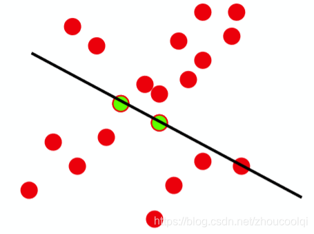
很显然,上述线性拟合的结果并不是我们想要的,我们真正需要的是一下拟合的效果:
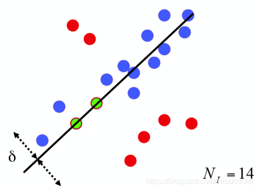
而这是RANSAC算法的拟合效果,因为剔除了不想被参与拟合的红点而选择在一定范围内的蓝点,这样保证了样本数据的干净,保证拟合效果更接近真实。
4.3 单应性矩阵
单应性矩阵可以由两幅图像(或者平面)中对应点对计算出来。每个对应点可以写出两个方程,分别对应与x和y坐标。因此,计算单应性矩阵H至少需要4对匹配点,过程如下:
那么就可以每次从所有的匹配点中选出4对,计算单应性矩阵,然后选出内点个数最多的作为最终的结果。计算距离方法如下:
(1)随机选择4对匹配特征对应点对
(2)根据DLT计算单应性矩阵H(唯一解)
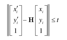
(3)对所有匹配点,计算映射误差(对每个对应点使用该单应性矩阵,然后返回平方距离之和)
(4)根据误差阈值,确定正常值inliers(小于阈值的点看做正确点,否则认为是错误的点)
重复步骤(1)-(4)
(5)针对最大inliers集合,重新计算单应性矩阵H
4.4 拼接图像
估计出单应性矩阵H后,我们需要将所有图像扭曲到一个公共的图像平面上。通常,这里的公共平面为中心平面(否则,需要进行大量变形)。一种方法是创建一个很大的图像,比如将平面中全部填充为0,使其和中心图像平行,然后将所有的图像扭曲到上面。其基本步骤如下:
(1)实现像素间的映射(计算像素和和单应性矩阵H相乘,然后对齐次坐标进行归一化)
(2)判断图像填补位置(查看H中的平移量,左边为正,右边为负)
(3)在单应性矩阵中加入平移量,进行alpha图填充
5.图像拼接实验步骤
5.1 检测并提取图像的特征和关键点
由sift特征提取提取图像的特征和关键角点,即'out_sift_1.txt'文件
5.2 匹配两个图像之间的描述符
from PIL import Image

# If you have PCV installed, these imports should work
from PCV.geometry import homography, warp

def match(desc1, desc2):
    """对于第一幅图像中的每个描述子,选取其在第二幅图像中的匹配
    输入:desc1(第一幅图像中的描述子),desc2(第二幅图像中的描述子)"""
    desc1 = array([d/linalg.norm(d) for d in desc1])
    desc2 = array([d/linalg.norm(d) for d in desc2])

    dist_ratio = 0.6
    desc1_size = desc1.shape
    matchscores = zeros((desc1_size[0],1),'int')
    desc2t = desc2.T #预先计算矩阵转置
    for i in range(desc1_size[0]):
        dotprods = dot(desc1[i,:],desc2t) #向量点乘
        dotprods = 0.9999*dotprods
        # 反余弦和反排序,返回第二幅图像中特征的索引
        indx = argsort(arccos(dotprods))

        #检查最近邻的角度是否小于dist_ratio乘以第二近邻的角度
        if arccos(dotprods)[indx[0]] < dist_ratio * arccos(dotprods)[indx[1]]:
            matchscores[i] = int(indx[0])

    return matchscores

def match_twosided(desc1, desc2):
    """双向对称版本的match()"""
    matches_12 = match(desc1, desc2)
    matches_21 = match(desc2, desc1)

    ndx_12 = matches_12.nonzero()[0]

    # 去除不对称的匹配
    for n in ndx_12:
        if matches_21[int(matches_12[n])] != n:
            matches_12[n] = 0

    return matches_12
5.3 使用RANSAC算法使用我们匹配的特征向量估计单应矩阵
5.3.1 构造单映性矩阵
from PCV.geometry import homography, warp

model = homography.RansacModel()
5.3.2 将匹配转换成齐次坐标点
# 将匹配转换成齐次坐标点的函数

def convert_points(j):
    ndx = matches[j].nonzero()[0]
    fp = homography.make_homog(l[j+1][ndx,:2].T)
    ndx2 = [int(matches[j][i]) for i in ndx]
    tp = homography.make_homog(l[j][ndx2,:2].T)

    # switch x and y - TODO this should move elsewhere
    fp = vstack([fp[1],fp[0],fp[2]])
    tp = vstack([tp[1],tp[0],tp[2]])
    return fp,tp

fp,tp = convert_points(0)
5.3.3 获取单应性矩阵和对应该单应性矩阵的正确点对
H_01 = homography.H_from_ransac(fp,tp,model)[0] class RansacModel(object):
""" 用于测试单应性矩阵的类,其中单应性矩阵是由网站
http://www.scipy.org/Cookbook/RANSAC上的ransac.py计算出来的"""
def __init__(self,debug=False):
self.debug = debug
def fit(self, data):
"""计算选取的4个对应的单应性矩阵 """
#将其转置,来调用H_from_points()计算单应性矩阵
data = data.T
# 映射的起始点
fp = data[:3,:4]
#映射的目标点
tp = data[3:,:4]
#计算单应性矩阵然后返回
return H_from_points(fp,tp)
def get_error( self, data, H):
"""对所有的对应计算单应性矩阵,然后对每个变换后的点,返回响应的误差"""
data = data.T
#映射的起始点
fp = data[:3]
#映射的目标点
tp = data[3:]
# 变换fp
fp_transformed = dot(H,fp)
# 归一化齐次坐标
fp_transformed = normalize(fp_transformed)
# 返回每个点的误差
return sqrt( sum((tp-fp_transformed)**2,axis=0) )
def H_from_ransac(fp,tp,model,maxiter=1000,match_theshold=10):
""" 使用RANSAC稳健性聚集点对应间的单应性矩阵H(ransac.py为从
http://www.scipy.org/Cookbook/RANSAC下载的版本).
输入: 齐次坐标表示的点fp,tp (3*n数组) """
from PCV.tools import ransac
# 对应点组
data = vstack((fp,tp))
# 计算H,并返回
H,ransac_data = ransac.ransac(data.T,model,4,maxiter,match_theshold,10,return_all=True)
return H,ransac_data['inliers']5.4 切割以及拼接图象
delta = 2000 # for padding and translation

im1 = array(Image.open(imname[0]), "uint8")

im2 = array(Image.open(imname[1]), "uint8")###
im_12 = warp.panorama(H_01,im1,im2,delta,delta)##
其中warp.panorama()用于图像扭曲。
def panorama(H,fromim,toim,padding=2400,delta=2400):
    """ 使用单应性矩阵H(使用RANSAC稳健性估计得出),协调两幅图像,创建水平全景图。结果
        为一幅和toim具有相同高度的图像。padding指定填充像素的数目,delta指定额外的平移量"""

    #检查图像是灰度图像,还是彩色图像
    is_color = len(fromim.shape) == 3

    # 用于geometric_transform()的单应性变换
    def transf(p):
        p2 = dot(H,[p[0],p[1],1])
        return (p2[0]/p2[2],p2[1]/p2[2])

    if H[1,2]<0: # fromim在右边
        print 'warp - right'
        # 变换fromim
        if is_color:
            # 在目标图像的右边填充0
            toim_t = hstack((toim,zeros((toim.shape[0],padding,3))))
            fromim_t = zeros((toim.shape[0],toim.shape[1]+padding,toim.shape[2]))
            for col in range(3):
                fromim_t[:,:,col] = ndimage.geometric_transform(fromim[:,:,col],
                                        transf,(toim.shape[0],toim.shape[1]+padding))
        else:
            # 在目标图像的右边填充0
            toim_t = hstack((toim,zeros((toim.shape[0],padding))))
            fromim_t = ndimage.geometric_transform(fromim,transf,
                                    (toim.shape[0],toim.shape[1]+padding))
    else:
        print 'warp - left'
        #为了补偿填充效果,在左边加入平移量
        H_delta = array([[1,0,0],[0,1,-delta],[0,0,1]])
        H = dot(H,H_delta)
        #fromim变换
        if is_color:
            # 在目标图像的左边填充0
            toim_t = hstack((zeros((toim.shape[0],padding,3)),toim))
            fromim_t = zeros((toim.shape[0],toim.shape[1]+padding,toim.shape[2]))
            for col in range(3):
                fromim_t[:,:,col] = ndimage.geometric_transform(fromim[:,:,col],
                                            transf,(toim.shape[0],toim.shape[1]+padding))
        else:
            # 在目标图像的左边填充0
            toim_t = hstack((zeros((toim.shape[0],padding)),toim))
            fromim_t = ndimage.geometric_transform(fromim,
                                    transf,(toim.shape[0],toim.shape[1]+padding))

    # 协调后返回(将fromim放在toim上)
    if is_color:
        # 所有非黑像素
        alpha = ((fromim_t[:,:,0] * fromim_t[:,:,1] * fromim_t[:,:,2] ) > 0)
        for col in range(3):
            toim_t[:,:,col] = fromim_t[:,:,col]*alpha + toim_t[:,:,col]*(1-alpha)
    else:
        alpha = (fromim_t > 0)
        toim_t = fromim_t*alpha + toim_t*(1-alpha)

    return toim_t
5.5 完整代码
修改sift.py以下代码两张图片的路径以及输出.txt文件名,运行得到out_sift_1.txt、out_sift_2.txt文件,然后运行后一段代码
#sift.py

from PIL import Image
#from numpy import *
from pylab import *
import os
import numpy as np
def process_image(imagename,resultname,params="--edge-thresh 10 --peak-thresh 5"):
    """ Process an image and save the results in a file. """

    if imagename[-3:] != 'pgm':
        # create a pgm file
        im = Image.open(imagename).convert('L')  #.convert('L') 将RGB图像转为灰度模式,灰度值范围[0,255]
        im.save('tmp.pgm')                       #将灰度值图像信息保存在.pgm文件中
        imagename = 'tmp.pgm'

    cmmd = str(r"F:/python/vlfeat-0.9.20/bin/win64/sift.exe "+imagename+" --output="+resultname+
                " "+params)
    os.system(cmmd)                              #执行sift可执行程序,生成resultname(test.sift)文件
    print('processed', imagename, 'to', resultname)


def read_features_from_file(filename):
    """ Read feature properties and return in matrix form. """
    #print(filename)
    f = np.loadtxt(filename)
    return f[:,:4],f[:,4:] # feature locations, descriptors


def plot_features(im,locs,circle=True):
    """ Show image with features. input: im (image as array),
        locs (row, col, scale, orientation of each feature). """

    def draw_circle(c,r):
        t = arange(0,1.01,.01)*2*pi
        x = r*cos(t) + c[0]
        y = r*sin(t) + c[1]
        plot(x,y,'b',linewidth=2)

    imshow(im)
    if circle:
        for p in locs:
            draw_circle(p[:2],p[2])
    else:
        plot(locs[:,0],locs[:,1],'ob')
    axis('off')


if __name__ == '__main__':
    imname = ('./screen/2/1.png')               #待处理图像路径
    #imname = ('./screen/2/2.png')
    im=Image.open(imname)
    process_image(imname,'out_sift_1.txt')
    l1,d1 = read_features_from_file('out_sift_1.txt')           #l1为兴趣点坐标、尺度和方位角度 l2是对应描述符的128 维向
    #process_image(imname,'out_sift_2.txt')
    #l1,d1 = read_features_from_file('out_sift_2.txt')
    figure()
    gray()
    plot_features(im,l1,circle = True)
    title('sift-features')
    show()
# -*- coding: utf-8 -*-
"""
Created on Sat Apr 23 15:36:26 2022

@author: 95490
"""

from pylab import *
from numpy import *
from PIL import Image

# If you have PCV installed, these imports should work
from PCV.geometry import homography, warp
from PCV.localdescriptors import sift

"""
This is the panorama example from section 3.3.
"""

def read_features_from_file(filename):
    """读取特征属性值,然后将其以矩阵的形式返回"""
    f = loadtxt(filename)
    return f[:,:4], f[:,4:] #特征位置,描述子

def write_featrues_to_file(filename, locs, desc):
    """将特征位置和描述子保存到文件中"""
    savetxt(filename, hstack((locs,desc)))

def plot_features(im, locs, circle=False):
    """显示带有特征的图像
       输入:im(数组图像),locs(每个特征的行、列、尺度和朝向)"""

    def draw_circle(c,r):
        t = arange(0,1.01,.01)*2*pi
        x = r*cos(t) + c[0]
        y = r*sin(t) + c[1]
        plot(x, y, 'b', linewidth=2)

    imshow(im)
    if circle:
        for p in locs:
            draw_circle(p[:2], p[2])
    else:
        plot(locs[:,0], locs[:,1], 'ob')
    axis('off')

def match(desc1, desc2):
    """对于第一幅图像中的每个描述子,选取其在第二幅图像中的匹配
    输入:desc1(第一幅图像中的描述子),desc2(第二幅图像中的描述子)"""
    desc1 = array([d/linalg.norm(d) for d in desc1])
    desc2 = array([d/linalg.norm(d) for d in desc2])

    dist_ratio = 0.6
    desc1_size = desc1.shape
    matchscores = zeros((desc1_size[0],1),'int')
    desc2t = desc2.T #预先计算矩阵转置
    for i in range(desc1_size[0]):
        dotprods = dot(desc1[i,:],desc2t) #向量点乘
        dotprods = 0.9999*dotprods
        # 反余弦和反排序,返回第二幅图像中特征的索引
        indx = argsort(arccos(dotprods))

        #检查最近邻的角度是否小于dist_ratio乘以第二近邻的角度
        if arccos(dotprods)[indx[0]] < dist_ratio * arccos(dotprods)[indx[1]]:
            matchscores[i] = int(indx[0])

    return matchscores

def match_twosided(desc1, desc2):
    """双向对称版本的match()"""
    matches_12 = match(desc1, desc2)
    matches_21 = match(desc2, desc1)

    ndx_12 = matches_12.nonzero()[0]

    # 去除不对称的匹配
    for n in ndx_12:
        if matches_21[int(matches_12[n])] != n:
            matches_12[n] = 0

    return matches_12

def appendimages(im1, im2):
    """返回将两幅图像并排拼接成的一幅新图像"""
    #选取具有最少行数的图像,然后填充足够的空行
    rows1 = im1.shape[0]
    rows2 = im2.shape[0]

    if rows1 < rows2:
        im1 = concatenate((im1, zeros((rows2-rows1,im1.shape[1]))),axis=0)
    elif rows1 >rows2:
        im2 = concatenate((im2, zeros((rows1-rows2,im2.shape[1]))),axis=0)
    return concatenate((im1,im2), axis=1)

def plot_matches(im1,im2,locs1,locs2,matchscores,show_below=True):
    """ 显示一幅带有连接匹配之间连线的图片
        输入:im1, im2(数组图像), locs1,locs2(特征位置),matchscores(match()的输出),
        show_below(如果图像应该显示在匹配的下方)
    """
    im3=appendimages(im1,im2)
    if show_below:
        im3=vstack((im3,im3))

    plt.figure(figsize=(20, 10))
    imshow(im3)

    cols1 = im1.shape[1]
    for i in range(len(matchscores)):
        if matchscores[i]>0:
            plot([locs1[i,0],locs2[matchscores[i,0],0]+cols1], [locs1[i,1],locs2[matchscores[i,0],1]],'c')
    axis('off')

# set paths to data folder
featname = ['out_sift_'+str(i+1)+'.txt' for i in range(2)]
imname = [str(i+1)+'.jpg' for i in range(2)]

# extract features and match
l = {}
d = {}

l[0],d[0] = read_features_from_file(featname[0])
l[1],d[1] = read_features_from_file(featname[1])
matches = {}

matches[0]  = match_twosided(d[1], d[0])##

# visualize the matches (Figure 3-11 in the book)

im1 = array(Image.open(imname[0]))
im2 = array(Image.open(imname[1]))
#figure()
#plot_matches(im2,im1,l[1],l[0],matches[0],show_below=True)


# function to convert the matches to hom. points
def convert_points(j):
    ndx = matches[j].nonzero()[0]
    fp = homography.make_homog(l[j+1][ndx,:2].T)
    ndx2 = [int(matches[j][i]) for i in ndx]
    tp = homography.make_homog(l[j][ndx2,:2].T)

    # switch x and y - TODO this should move elsewhere
    fp = vstack([fp[1],fp[0],fp[2]])
    tp = vstack([tp[1],tp[0],tp[2]])
    return fp,tp

# estimate the homographies
model = homography.RansacModel()

fp,tp = convert_points(0)
H_01 = homography.H_from_ransac(fp,tp,model)[0] #im 0 to 1


# warp the images
delta = 2000 # for padding and translation

im1 = array(Image.open(imname[0]), "uint8")

im2 = array(Image.open(imname[1]), "uint8")###
im_12 = warp.panorama(H_01,im1,im2,delta,delta)##

figure()
imshow(array(im_12, "uint8"))
axis('off')
show()
5.6 实验结果
