1.实验原理
(1)RANSAC算法
采用RANSAC算法寻找一个最佳单应性矩阵H,矩阵大小为3×3。RANSAC目的是找到最优的参数矩阵使得满足该矩阵的数据点个数最多,通常令h33=1来归一化矩阵。由于单应性矩阵有8个未知参数,至少需要8个线性方程求解,对应到点位置信息上,一组点对可以列出两个方程,则至少包含4组匹配点对。
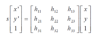
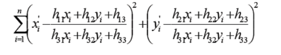
RANSAC算法从匹配数据集中随机抽出4个样本并保证这4个样本之间不共线,计算出单应性矩阵,然后利用这个模型测试所有数据,并计算满足这个模型数据点的个数与投影误差(即代价函数),若此模型为最优模型,则对应的代价函数最小。
RANSAC算法步骤:
1. 随机从数据集中随机抽出4个样本数据 (此4个样本之间不能共线),计算出变换矩阵H,记为模型M;
2. 计算数据集中所有数据与模型M的投影误差,若误差小于阈值,加入内点集 I ;
3. 如果当前内点集 I 元素个数大于最优内点集 I_best , 则更新 I_best = I,同时更新迭代次数k ;
4. 如果迭代次数大于k,则退出 ; 否则迭代次数加1,并重复上述步骤;
(2)图像配准
图像配准是图像处理研究领域中的一个典型问题和技术难点,其目的在于比较或融合针对同一对象在不同条件下获取的图像,例如图像会来自不同的采集设备,取自不同的时间,不同的拍摄视角等等,有时也需要用到针对不同对象的图像配准问题。具体地说,对于一组图像数据集中的两幅图像,通过寻找一种空间变换把一幅图像映射到另一幅图像,使得两图中对应于空间同一位置的点一一对应起来,从而达到信息融合的目的。 基于特征的匹配方法是图像配准中的一类方法,首先提取图像的特征,再生成特征描述子,最后根据描述子的相似程度对两幅图像的特征之间进行匹配。图像的特征主要可以分为点、线(边缘)、区域(面)等特征,也可以分为局部特征和全局特征。区域(面)特征提取比较麻烦,耗时,因此主要用点特征和边缘特征。
具体可参考https://blog.csdn.net/gaoyu1253401563/article/details/80631601
关于Apap图像配准算法的实现流程:
1.提取两张图片的sift特征点
2.对两张图片的特征点进行粗匹配,再用RANSAC的改进算法进行特征点对的筛选。筛选后的特征点基本能够一一对应。
3.使用DLT算法(直接线性法)将剩下的特征点对进行透视变换矩阵的估计。
4.由于此时得到的透视变换矩阵是基于全局特征点对进行的,通常为了提高精确度,Apap将图像切割成无数多个小方块,对每个小方块的变换矩阵逐一估计。
(3)图像分割
原文:https://imlogm.github.io/图像处理/mincut-maxflow/
关于最小割(min-cut)
如图所示,是一个有向带权图,共有4个顶点和5条边。
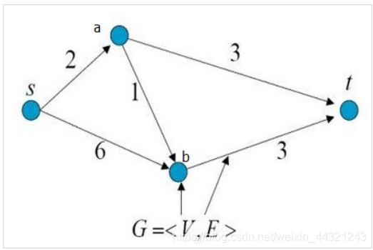
图中顶点s表示源点(source),顶点t表示终点(terminal),从源点s到终点t共有3条路径:
s -> a -> t
s -> b -> t
s -> a -> b-> t
现在要求剪短图中的某几条边,使得不存在从s到t的路径,并且保证所减的边的权重和最小。
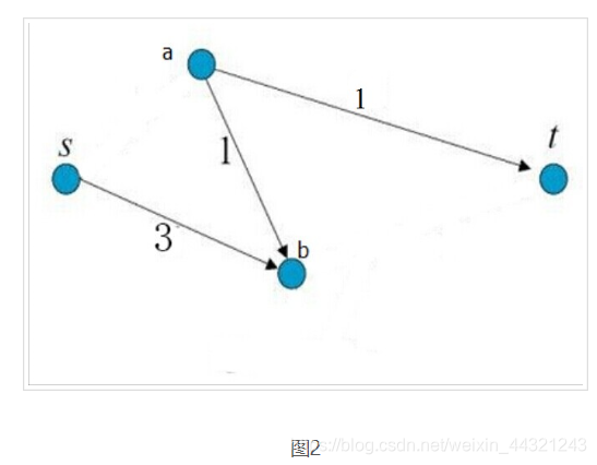
剪完以后的图如下图所示。所修剪的边的权重和为:2 + 3 = 5,为所有修剪方式中权重和最小的。
这样的修剪称为最小割。
关于最大流(max-flow)
继续以图1为例,假如顶点s源源不断有水流出,边的权重代表该边允许通过的最大水流量,求顶点t流入的最大水流量
从s到t的3条路径:
s -> a -> t:流量被边”s -> a”限制,最大流量为2
s -> b -> t:流量被边”b -> t”限制,最大流量为3
s -> a -> b-> t:边”s -> a”的流量已经被其他路径占满,没有流量
所以,顶点t能够流入的最大水流量为:2 + 3 = 5。最大流为:2 + 3 = 5。
(4)图像融合
相关代码:(采用alpha blending。利用alpha通道,实现图像的两两融合。
)
def panorama(H,fromim,toim,padding=2400,delta=2400):
    """ Create horizontal panorama by blending two images
        using a homography H (preferably estimated using RANSAC).
        The result is an image with the same height as toim. 'padding'
        specifies number of fill pixels and 'delta' additional translation. """


# check if images are grayscale or color
is_color = len(fromim.shape) == 3

# homography transformation for geometric_transform()
def transf(p):
    p2 = dot(H,[p[0],p[1],1])
    return (p2[0]/p2[2],p2[1]/p2[2])

if H[1,2]<0: # fromim is to the right
    print ('warp - right')
    # transform fromim
    if is_color:
        # pad the destination image with zeros to the right
        toim_t = hstack((toim,zeros((toim.shape[0],padding,3))))
        fromim_t = zeros((toim.shape[0],toim.shape[1]+padding,toim.shape[2]))
        for col in range(3):
            fromim_t[:,:,col] = ndimage.geometric_transform(fromim[:,:,col],
                                    transf,(toim.shape[0],toim.shape[1]+padding))
    else:
        # pad the destination image with zeros to the right
        toim_t = hstack((toim,zeros((toim.shape[0],padding))))
        fromim_t = ndimage.geometric_transform(fromim,transf,
                                (toim.shape[0],toim.shape[1]+padding))
else:
    print ('warp - left')
    # add translation to compensate for padding to the left
    H_delta = array([[1,0,0],[0,1,-delta],[0,0,1]])
    H = dot(H,H_delta)
    # transform fromim
    if is_color:
        # pad the destination image with zeros to the left
        toim_t = hstack((zeros((toim.shape[0],padding,3)),toim))
        fromim_t = zeros((toim.shape[0],toim.shape[1]+padding,toim.shape[2]))
        for col in range(3):
            fromim_t[:,:,col] = ndimage.geometric_transform(fromim[:,:,col],
                                        transf,(toim.shape[0],toim.shape[1]+padding))
    else:
        # pad the destination image with zeros to the left
        toim_t = hstack((zeros((toim.shape[0],padding)),toim))
        fromim_t = ndimage.geometric_transform(fromim,
                                transf,(toim.shape[0],toim.shape[1]+padding))

# blend and return (put fromim above toim)
if is_color:
    # all non black pixels
    alpha = ((fromim_t[:,:,0] * fromim_t[:,:,1] * fromim_t[:,:,2] ) > 0)
    for col in range(3):
        toim_t[:,:,col] = fromim_t[:,:,col]*alpha + toim_t[:,:,col]*(1-alpha)
else:
    alpha = (fromim_t > 0)
    toim_t = fromim_t*alpha + toim_t*(1-alpha)

return toim_t
**alpha=1 得到当前图片
alpha=0 得到黑色预设背景
2.实验代码
# -*- coding: utf-8 -*-
from pylab import *
from numpy import *
from PIL import Image

# If you have PCV installed, these imports should work
from PCV.geometry import homography, warp
from PCV.localdescriptors import sift

"""
This is the panorama example from section 3.3.
"""

# set paths to data folder
featname = ['im' + str(i + 1) + '.sift' for i in range(5)]  # 图片路径记得修改
imname = ['im' + str(i + 1) + '.jpg' for i in range(5)]

# extract features and match
l = {}
d = {}
for i in range(5):
    sift.process_image(imname[i], featname[i])
    l[i], d[i] = sift.read_features_from_file(featname[i])

matches = {}
for i in range(4):
    matches[i] = sift.match(d[i + 1], d[i])

# visualize the matches (Figure 3-11 in the book)
for i in range(4):
    im1 = array(Image.open(imname[i]))
    im2 = array(Image.open(imname[i + 1]))
    figure()
    sift.plot_matches(im2, im1, l[i + 1], l[i], matches[i], show_below=True)


# function to convert the matches to hom. points
def convert_points(j):
    ndx = matches[j].nonzero()[0]
    fp = homography.make_homog(l[j + 1][ndx, :2].T)
    ndx2 = [int(matches[j][i]) for i in ndx]
    tp = homography.make_homog(l[j][ndx2, :2].T)

    # switch x and y - TODO this should move elsewhere
    fp = vstack([fp[1], fp[0], fp[2]])
    tp = vstack([tp[1], tp[0], tp[2]])
    return fp, tp


# estimate the homographies
model = homography.RansacModel()

fp, tp = convert_points(1)
H_12 = homography.H_from_ransac(fp, tp, model)[0]  # im 1 to 2

fp, tp = convert_points(0)
H_01 = homography.H_from_ransac(fp, tp, model)[0]  # im 0 to 1

tp, fp = convert_points(2)  # NB: reverse order
H_32 = homography.H_from_ransac(fp, tp, model)[0]  # im 3 to 2

tp, fp = convert_points(3)  # NB: reverse order
H_43 = homography.H_from_ransac(fp, tp, model)[0]  # im 4 to 3

# warp the images
delta = 2000  # for padding and translation

im1 = array(Image.open(imname[1]), "uint8")
im2 = array(Image.open(imname[2]), "uint8")
im_12 = warp.panorama(H_12, im1, im2, delta, delta)

im1 = array(Image.open(imname[0]), "f")
im_02 = warp.panorama(dot(H_12, H_01), im1, im_12, delta, delta)

im1 = array(Image.open(imname[3]), "f")
im_32 = warp.panorama(H_32, im1, im_02, delta, delta)

im1 = array(Image.open(imname[4]), "f")
im_42 = warp.panorama(dot(H_32, H_43), im1, im_32, delta, 2 * delta)

figure()
imshow(array(im_42, "uint8"))
axis('off')
savefig("example1.png", dpi=300)
imsave('im.jpg', array(im_42, "uint8"))
show()
实验结果
ps:针对不同的常见图片作拼接
1.景深落差大的情况
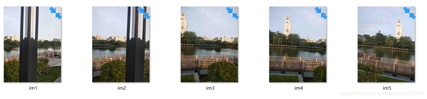
拼接结果

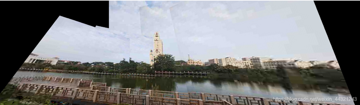
误差分析:
由于拍摄角度问题,原本直立的景象拼合后变成倾斜。
曝光不均导致全景图像画面分割明显。
景深落差小的情况
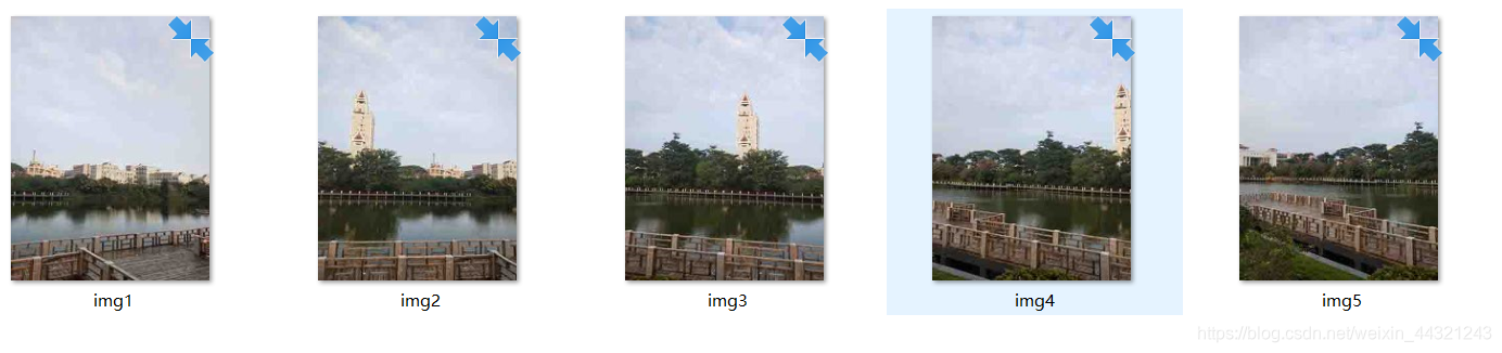
拼接结果:
室内:
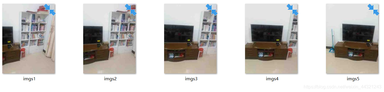
拼接结果:
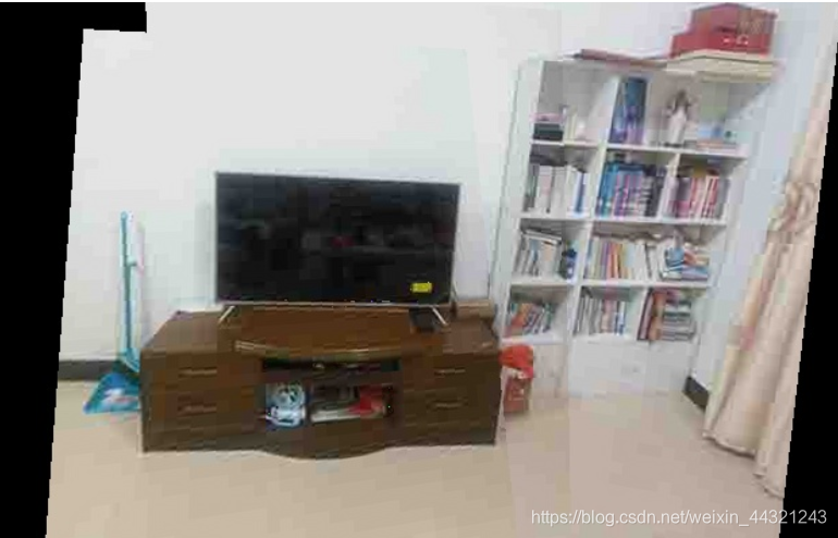
分析:
分割稍不明显,拼合效果较好。