相关环境的搭建
1、PCV
2、VLFeat工具包
3、pydot
这里大家可以移步我另外一个博客
https://blog.csdn.net/zxm_jimin/article/details/88596987
原理部分
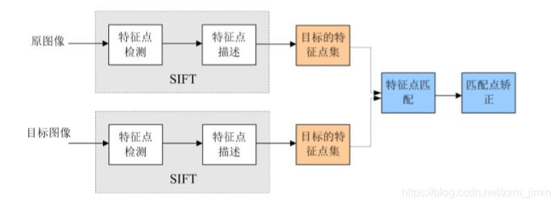
特征匹配基本流程
根据准则,提取图像中的特征点
提取特征点周围的图像块,构造特征描述符
通过特征描述符对比,实现特征匹配
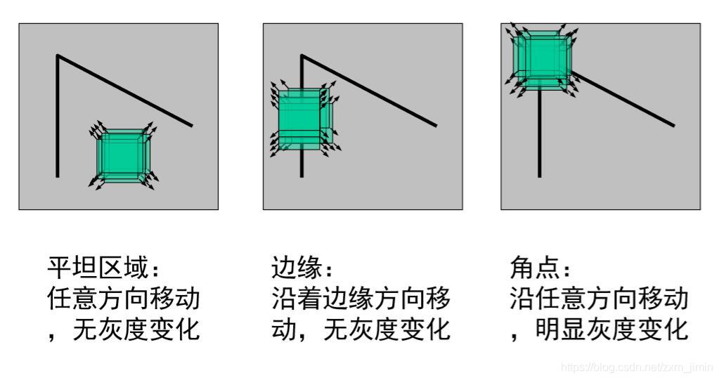
角点(corner points):即特征点
• 局部窗口沿各方向移动,均产生明显变化的点
• 图像局部曲率突变的点
首先我们先来了解一下
Harris角点检测算法
该算法的主要思想是,如果像素周围显示存在多于一个方向的边,我们认为该点为兴趣点,即角点。
HARRIS角点检测基本思想
• 从图像局部的小窗口观察图像特征
• 角点定义 <–窗口向任意方向的移动都导致图像灰度的明显变化
(像素周围显示存在多于一个方向的边)
这里不对Harris算法做过多介绍,但我们知道。它检测出来的特征点是不具有尺度不变性和方向不变性的。因此,即使两张图片的拍摄角度变化,也不能找到对应的特征点。
这种情况下,我们使用SIFT算法。
SIFT(尺度不变特征变换)
SIFT算法可以解决的问题:
• 目标的旋转、缩放、平移(RST)
• 图像仿射/投影变换(视点viewpoint)
• 弱光照影响(illumination)
• 部分目标遮挡(occlusion)
• 杂物场景(clutter)
• 噪声
SIFT算法实现
SIFT算法的实质可以归为在不同尺度空间上查找特征点(关键点)的问题。
主要有三个流程:
1、提取关键点;
2、对关键点附加 详细的信息(局部特征),即描述符;
3、通过特征点(附带上特征向量的关键点)的两两比较找出相互匹配的若干对特征点,建立景物间的对应关系。
兴趣点
我们希望选出具有以下不变性的点:尺度 方向 位移 光照
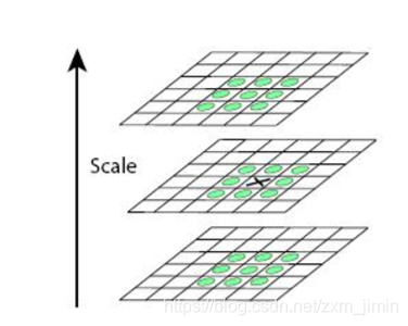
尺度不变性
尺度空间理论最早于1962年提出,其主要思想是通过对原始图像进行尺度变换,获得图像多尺度下的空间表示。从而实现边缘、角点检测和不同分辨率上的特征提取,以满足特征点的尺度不变性。
尺度空间中各尺度图像的 模糊程度逐渐变大,能够模拟人在距离目标由近到远时目标在视网膜上的形成过程。
尺度越大图像越模糊

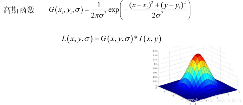
目前已知,高斯核是唯一可以产生 多尺度空间的核,一个 图像的尺度空间,L(x, y, σ) ,定义为原始图像 I(x, y)与一个可变尺度的2 维高斯函数G(x, y, σ) 卷积运算
σ越大,则保留边缘,因为将周围点纳入考虑的程度大。
σ越小,则保留细节,因为将周围点纳入考虑的程度小。
高斯金字塔
高斯金子塔的构建过程可分为两步:
(1)对图像做高斯平滑;
(2)对图像做降采样。
为了让尺度体现其连续性,在简单下采样的基础上加上了高斯滤波。一幅图像可以产生几组(octave)图像,一组图像包括几层(interval)图像。
但我们知道,直接使用此方法,会导致计算量过大,因此,我们采用另一种更高效的方法——DOG高斯差分金字塔
对应DOG算子,需构建DOG金字塔
可以通过高斯差分图 像看出图像上的像素值变化情况。(如果没有变化,也就没有特征。特征必须是变化尽可能多的点。) DOG图像描绘的是目标的轮廓。

DOG的局部极值点
我们知道,其实在角点附近的点也可能具有很大的变化,因此,我们要从中取最优。
在DOG空间下的(上中下)三层列入考虑范围,寻找局部最大点。以确保在尺度空间和二维图像空间都检测到极值点。
去除边缘响应
由于DOG函数在图像边缘有较强的边缘响应,因此需要排除边缘响应。
DOG函数的峰值点在边缘方向有较大的主曲率,而在垂直边缘的方向有 较小的主曲率。主曲率可以通过计算在该点位置尺度的2×2的Hessian矩 阵得到,导数由采样点相邻差来估计:


旋转不变性
通过尺度不变性求极值点,可以使其具有缩放不变的性质。而利用关键点邻域像素的梯度方向分布特性,可以为每个关键点指定方向参数方向,从而使描述子对图像旋转具有不变性。
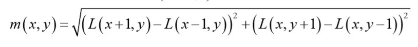
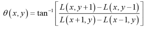
通过求出每个极值点的梯度来为极值点赋予方向。
像素点的梯度表示
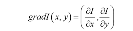
梯度幅值:(两点之间的变化)
梯度方向:利用三角函数(arctanX)求出角度
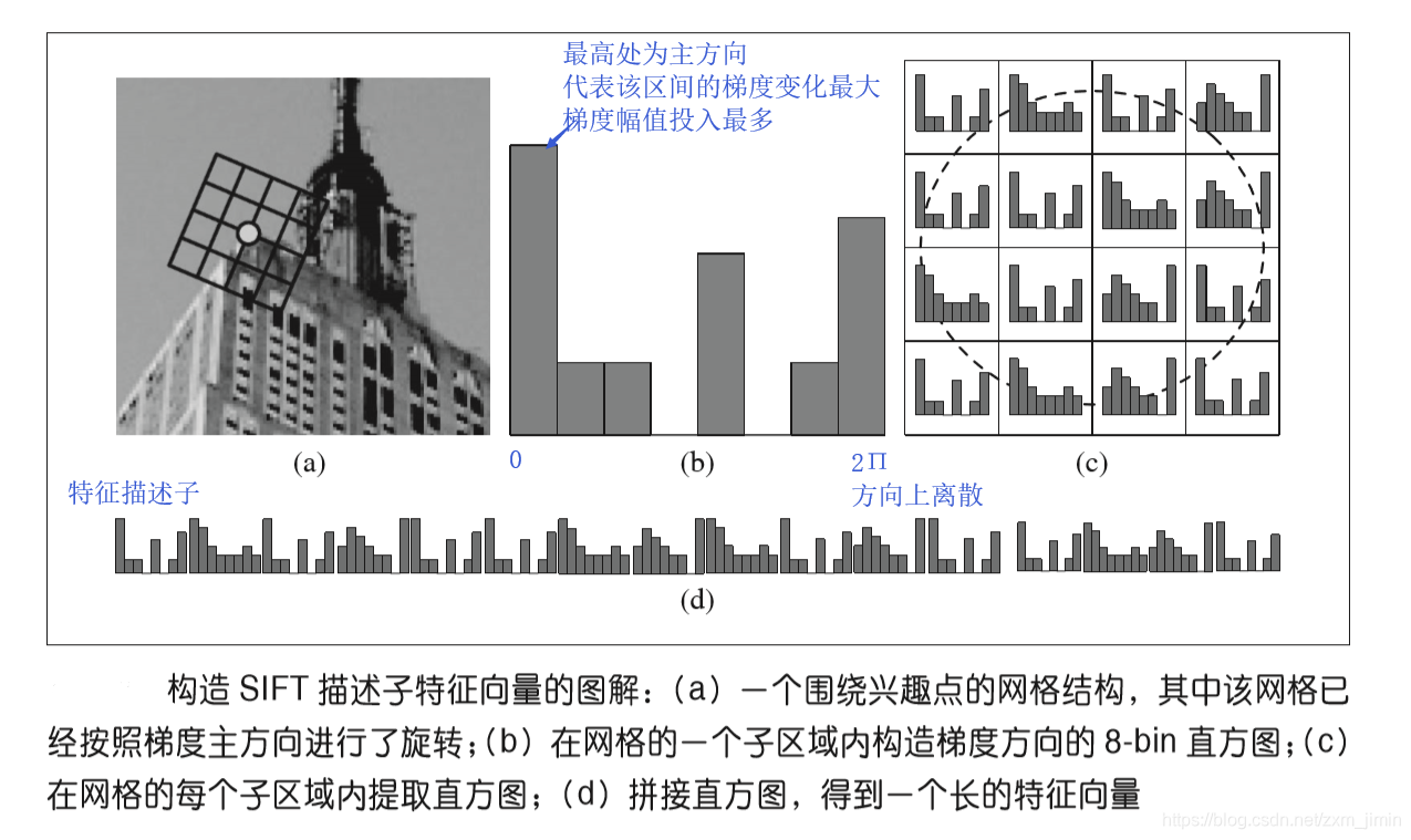
确定关键点的方向采用梯度直方图统计法,统计以关键点为原点,一定区域内的图像像素点对关键点方向生成所作的贡献。
• 关键点主方向:极值点周围区域梯度直方图的主峰值也是特征点方向
• 关键点辅方向:在梯度方向直方图中,当存在另一个相当于主峰值 80%能量的峰值时,则将这个方向认为是该关键点的辅方向。
这可以增强匹配的鲁棒性,Lowe的论文指出大概有15%关键点具有 多方向,但这些点对匹配的稳定性至为关键。
以关键点的主方向切割像素块
SIFT 描述子在每个像素点附近选取子区域网格,在每个子区域内计算图像 梯度方向直方图。每个子区域的直方图拼接起来组成描述子向量。SIFT 描述子的标 准设置使用 4×4 的子区域,每个子区域使用 8 个小区间的方向直方图,会产生共 128 个小区间的直方图(4×4×8=128)。所示为描述子的构造过程。
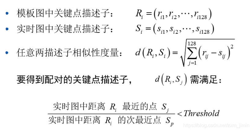
匹配描述子
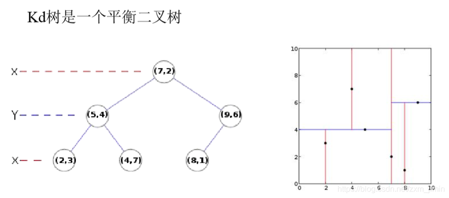
关键点的匹配可以采用穷举法来完成,但是这样耗费的时间太多,一般都采用kd树的数据结构来完成搜索。
搜索的内容是以目标图像的关键点为基准,搜索与目标图像的特征点最邻近的原图像特征点和次邻近的原图像特征点。
原理部分结束。
实验部分
接下来我们来看看如何用代码来实现:
在PCV中的 sift.py
VLFeat 库是用 C 语言来写的,但是我们可以使用该库提供的命令行接口。
处理一幅图像,然后将结果保存在文件中

def process_image(imagename,resultname,params="--edge-thresh 10 --peak-thresh 5"):
    """ process an image and save the results in a file"""
    if imagename[-3:] != 'pgm':
	    #create a pgm file
		 im = Image.open(imagename).convert('L')
		 im.save('tmp.pgm')
		 imagename = 'tmp.pgm'
    cmmd = str(path+imagename+" --output="+resultname+
				" "+params)
    os.system(cmmd)
    print('processed', imagename, 'to', resultname)
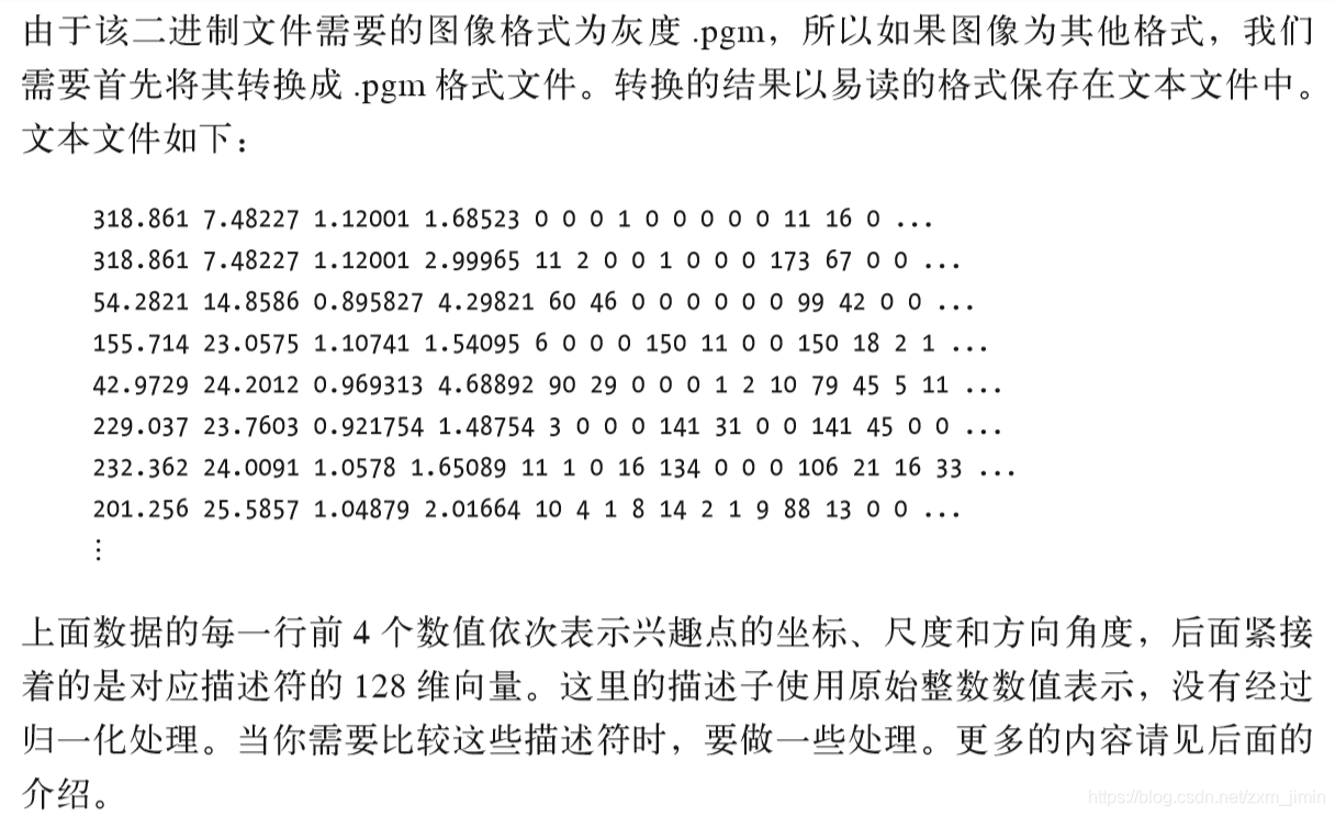
读取特征属性值,然后将其以矩阵的形式返回
    def read_features_from_file(filename):
	""" read feature properties and return in matrix form"""
	f = loadtxt(filename)
	return f[:,:4],f[:,4:] # feature locations, descriptors
将特征位置和描述子保存到文件中
此函数使用了 hstack() 函数。该函数通过拼接不同的行向量来实现水平堆叠两个向量的功能。在这个例子中,每一行中前几列为位置信息,紧接着是描述子。
def write_features_to_file(filename,locs,desc):
	""" save feature location and descriptor to file"""
	savetxt(filename,hstack((locs,desc)))
显示带有特征的图像
该函数在原始图像上使用蓝色的点绘制出 SIFT 特征点的位置。将参数 circle 的选项设置为 True,该函数将使用 draw_circle() 函数绘制出圆圈,圆圈的半径为特征的尺度
def plot_features(im,locs,circle=False):
	""" show image with features. input: im (image as array),
		locs (row, col, scale, orientation of each feature)
		 输入:im(数组图像),locs(每个特征的行、列、尺度和朝向) """

def draw_circle(c,r):
	t = arange(0,1.01,.01)*2*pi
	x = r*cos(t) + c[0]
	y = r*sin(t) + c[1]
	plot(x,y,'b',linewidth=2)

imshow(im)
if circle:
	[draw_circle([p[0],p[1]],p[2]) for p in locs]
else:
	plot(locs[:,0],locs[:,1],'ob')
axis('off')
匹配函数
对于将一幅图像中的特征匹配到另一幅图像的特征,一种稳健的准则(同样是由 Lowe 提出的)是使用这两个特征距离和两个最匹配特征距离的比率。相比于图像中的其他特征,该准则保证能够找到足够相似的唯一特征。使用该方法可以使错误的匹配数降低。
该函数使用描述子向量间的夹角作为距离度量。在此之前,我们需要将描述子向量 归一化到单位长度 1。因为这种匹配是单向的,即我们将每个特征向另一幅图像中的 所有特征进行匹配,所以我们可以先计算第二幅图像兴趣点描述子向量的转置矩阵。 这样,我们就不需要对每个特征分别进行转置操作。
def match(desc1,desc2):
	""" for each descriptor in the first image,
		select its match in the second image.
		input: desc1 (descriptors for the first image),
		desc2 (same for second image).
		对于第一幅图像中的每个描述子,选取其在第二幅图像中的匹配
		 输入:desc1(第一幅图像中的描述子),desc2(第二幅图像中的描述子)"""

desc1 = array([d/linalg.norm(d) for d in desc1])
desc2 = array([d/linalg.norm(d) for d in desc2])

dist_ratio = 0.6
desc1_size = desc1.shape

matchscores = zeros((desc1_size[0],1))
desc2t = desc2.T #precompute matrix transpose 预先计算矩阵转置
for i in range(desc1_size[0]):
	dotprods = dot(desc1[i,:],desc2t) #vector of dot products  向量点乘
	dotprods = 0.9999*dotprods
	#inverse cosine and sort, return index for features in second image
	 # 反余弦和反排序,返回第二幅图像中特征的索引
	indx = argsort(arccos(dotprods))

	#check if nearest neighbor has angle less than dist_ratio times 2nd
	# 检查最近邻的角度是否小于 dist_ratio 乘以第二近邻的角度
	if arccos(dotprods)[indx[0]] < dist_ratio * arccos(dotprods)[indx[1]]:
		matchscores[i] = int(indx[0])

return matchscore
Harris和sift特征匹配处理 结果对比
寻找特征点
ch2_harris_sift.py
    # 添加中文字体支持
    from matplotlib.font_manager import FontProperties
    font = FontProperties(fname=r"c:\windows\fonts\SimSun.ttc", size=14)

    imname = '../mydata/test1.jpg'
    im = array(Image.open(imname).convert('L'))
    sift.process_image(imname, 'test1.sift')
    l1, d1 = sift.read_features_from_file('test1.sift')

    figure()
    gray()
    subplot(131)
    sift.plot_features(im, l1, circle=False)
    title(u'SIFT特征',fontproperties=font)
    subplot(132)
    sift.plot_features(im, l1, circle=True)
    title(u'用圆圈表示SIFT特征尺度',fontproperties=font)

    # 检测harris角点
    harrisim = harris.compute_harris_response(im)

    subplot(133)
    filtered_coords = harris.get_harris_points(harrisim, 6, 0.1)
    imshow(im)
    plot([p[1] for p in filtered_coords], [p[0] for p in filtered_coords], '*')
    axis('off')
    title(u'Harris角点',fontproperties=font)

    show()
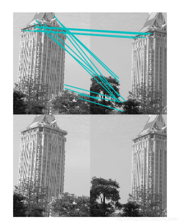
sift特征匹配处理
ch2_sift_match.py

from PIL import Image
from pylab import *
import sys
from PCV.localdescriptors import sift
import numpy as np

if len(sys.argv) >= 3:
  im1f, im2f = sys.argv[1], sys.argv[2]
else:

  im1f = '../mydata/test1.jpg'
  im2f = '../mydata/test2.jpg'

im1 = array(Image.open(im1f))
im2 = array(Image.open(im2f))

sift.process_image(im1f, 'out_sift_1.txt')
l1, d1 = sift.read_features_from_file('out_sift_1.txt')
figure()
gray()
subplot(121)
sift.plot_features(im1, l1, circle=False)

sift.process_image(im2f, 'out_sift_2.txt')
l2, d2 = sift.read_features_from_file('out_sift_2.txt')
subplot(122)
sift.plot_features(im2, l2, circle=False)

#matches = sift.match(d1, d2)
matches = sift.match_twosided(d1, d2)
print('{} matches'.format(len(matches.nonzero()[0])))

figure()
gray()

# l4 = l2.astype(np.int8)
l3 = l1.astype('int')
l4 = l2.astype('int')


list(l3)
list(l4)
print(l3.tolist())
print(l4.tolist())
sift.plot_matches(im1, im2, l3, l4, matches, show_below=True)
show()
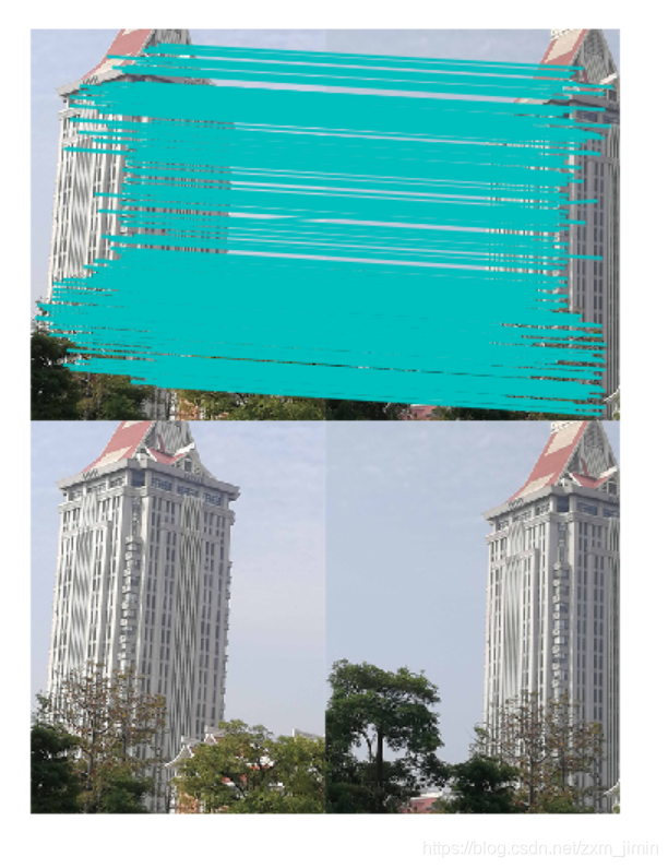
Harris特征匹配处理
 # -*- coding: utf-8 -*-
from pylab import *
from PIL import Image

from PCV.localdescriptors import harris
from PCV.tools.imtools import imresize

"""
This is the Harris point matching example in Figure 2-2.
"""

im1 = array(Image.open("../mydata/test1.jpg").convert("L"))
im2 = array(Image.open("../mydata/test2.jpg").convert("L"))
# resize加快匹配速度

# TypeError: integer argument expected, got float

# cv2.resize内的参数是要求为整数
# “/”改为“//”运算
im1 = imresize(im1, (im1.shape[1]//2, im1.shape[0]//2))
im2 = imresize(im2, (im2.shape[1]//2, im2.shape[0]//2))

wid = 5
harrisim = harris.compute_harris_response(im1, 5)
filtered_coords1 = harris.get_harris_points(harrisim, wid+1)
d1 = harris.get_descriptors(im1, filtered_coords1, wid)

harrisim = harris.compute_harris_response(im2, 5)
filtered_coords2 = harris.get_harris_points(harrisim, wid+1)
d2 = harris.get_descriptors(im2, filtered_coords2, wid)

print('starting matching')
matches = harris.match_twosided(d1, d2)

figure()
gray()

harris.plot_matches(im1, im2, filtered_coords1, filtered_coords2, matches)
show()
比较的这两张图片是集美大学的尚大楼,图片拍摄角度有轻微旋转
可以明显看出,sift算法的效果更好
因为它更好的处理了旋转不变性,而Harris算法的描述子中并未考虑到方向。
集美大学小地图
算法流程:
先对目录下的所有图片做sift处理
设定一个匹配成功的阈值
然后循环遍历图片列表,先两两匹配,若匹配成功(匹配的数目高于阈值)则画出图像节点及其连线
# -*- coding: utf-8 -*-
from PIL import Image
from pylab import *
from numpy import *
import os
import pydot
from PCV.localdescriptors import sift


def get_imlist(path):
    return [os.path.join(path, f) for f in os.listdir(path) if f.endswith('.jpg')]


# pydot需要绝对路径
download_path = "D:\workspace\Computer Vision\\test1\mydata\jmu"
path = "D:\workspace\Computer Vision\\test1\mydata\jmu"

# list of downloaded filenames
imlist = get_imlist(download_path)
nbr_images = len(imlist)

# extract features
featlist = [imname[:-3] + 'sift' for imname in imlist]
for i, imname in enumerate(imlist):
    sift.process_image(imname, featlist[i])

matchscores = zeros((nbr_images, nbr_images))

for i in range(nbr_images):
    for j in range(i, nbr_images):  # only compute upper triangle
        print('comparing ', imlist[i], imlist[j])
        l1, d1 = sift.read_features_from_file(featlist[i])
        l2, d2 = sift.read_features_from_file(featlist[j])
        matches = sift.match_twosided(d1, d2)
        nbr_matches = sum(matches > 0)
        print( 'number of matches = ', nbr_matches)
        matchscores[i, j] = nbr_matches
print("The match scores is: \n", matchscores)

# copy values
for i in range(nbr_images):
    for j in range(i + 1, nbr_images):  # no need to copy diagonal
        matchscores[j, i] = matchscores[i, j]

# 可视化
threshold = 2  # min number of matches needed to craete link

g = pydot.Dot(graph_type='graph')  # don't want the default directed graph

for i in range(nbr_images):
    for j in range(i + 1, nbr_images):
        if matchscores[i, j] > threshold:
            # 图像对中的第一幅图像
            im = Image.open(imlist[i])
            im.thumbnail((100, 100))
            filename = path + str(i) + '.png'
            im.save(filename)  # 需要一定大小的临时文件
            g.add_node(pydot.Node(str(i), fontcolor='transparent',
                                  shape='rectangle', image=filename))

            # 图像对中的第二幅图像
            im = Image.open(imlist[j])
            im.thumbnail((100, 100))
            filename = path + str(j) + '.png'
            im.save(filename)  # 需要一定大小的临时文件
            g.add_node(pydot.Node(str(j), fontcolor='transparent',
                                  shape='rectangle', image=filename))
            g.add_edge(pydot.Edge(str(i), str(j)))
g.write_png('jmu.png')
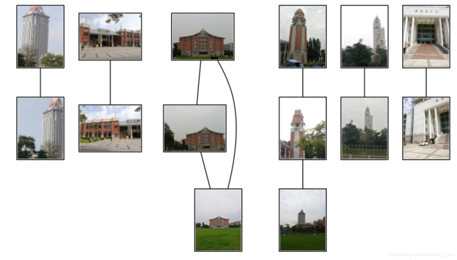
匹配结果:
总共放入15张图片,有14张图片成功匹配 ;匹配出6对图片
可以看出sift算法对
• 目标的旋转、缩放、平移(RST)
• 图像仿射/投影变换(视点viewpoint)
• 弱光照影响(illumination)
• 部分目标遮挡(occlusion)
• 杂物场景(clutter)
• 噪声
确实有很好的效果
这归功于,sift 特征点具有尺度、方向、位移、光照的不变性。
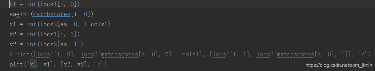
PS:
PCV中的sift.py下的此函数好像有问题
def plot_matches(im1, im2, locs1, locs2, matchscores, show_below=True):
会报错
IndexError:arrays used as indices must be of integer (or boolean) type
问题解决
因为画图时使用[ ]来标定,所以一定要是整数类型
而 locs1, locs2, matchscores存放的都是float类型
在百度并尝试后,发现:
matchscores.astype(int)
matchscores.astype(‘int’)
matchscores.astype(‘int32’)
这些方法都不可行
因为源文件中没有改变
所以最后采用
可以使用。