We've put the notebooks that you used this week into GitHub so you can download and play with them.

What are convolutions and pooling?

In the previous example, you saw how you could create a neural network called a deep neural network to pattern match a set of images of fashion items to labels. In just a couple of minutes, you're able to train it to classify with pretty high accuracy on the training set, but a little less on the test set. Now, one of the things that you would have seen when you looked at the images is that there's a lot of wasted space in each image. While there are only 784 pixels, it will be interesting to see if there was a way that we could condense the image down to the important features that distinguish what makes it a shoe, or a handbag, or a shirt. That's where convolutions come in.

So, what's convolution? You might ask.

Well, if you've ever done any kind of image processing, it usually involves having a filter and passing that filter over the image in order to change the underlying image. The process works a little bit like this. For every pixel, take its value, and take a look at the value of its neighbors. If our filter is three by three, then we can take a look at the immediate neighbor, so that you have a corresponding three by three grid. Then to get the new value for the pixel, we simply multiply each neighbor by the corresponding value in the filter. So, for example, in this case, our pixel has the value 192, and its upper left neighbor has the value zero. The upper left value and the filter is a negative one, so we multiply zero by negative one. Then we would do the same for the upper neighbor. Its value is 64 and the corresponding filter value was zero, so we'd multiply those out. Repeat this for each neighbor and each corresponding filter value, and would then have the new pixel with the sum of each of the neighbor values multiplied by the corresponding filter value, and that's a convolution. It's really as simple as that.

The idea here is that some convolutions will change the image in such a way that certain features in the image get emphasized.

So, for example, if you look at this filter, then the vertical lines in the image really pop out. With this filter, the horizontal lines pop out. Now, that's a very basic introduction to what convolutions do, and when combined with something called pooling, they can become really powerful.

But simply, pooling is a way of compressing an image.

A quick and easy way to do this is to go over the image of four pixels at a time, i.e, the current pixel and its neighbors underneath and to the right of it. Of these four, pick the biggest value and keep just that. So, for example, you can see it here. My 16 pixels on the left are turned into the four pixels on the right, by looking at them in two-by-two grids and picking the biggest value. This will preserve the features that were highlighted by the convolution, while simultaneously quartering the size of the image. We have horizontal and vertical axes.

The concepts introduced in this video are available as Conv2D layers and MaxPooling2D layers in TensorFlow. You’ll learn how to implement them in code in the next video…

tf.keras.layers.Conv2D(2.0)

Arguments:

filters: Integer, the dimensionality of the output space (i.e. the number of output filters in the convolution).

kernel_size: An integer or tuple/list of 2 integers, specifying the height and width of the 2D convolution window. Can be a single integer to specify the same value for all spatial dimensions.

strides: An integer or tuple/list of 2 integers, specifying the strides of the convolution along the height and width. Can be a single integer to specify the same value for all spatial dimensions. Specifying any stride value != 1 is incompatible with specifying any dilation_rate value != 1.

padding: one of "valid" or "same" (case-insensitive).

data_format: A string, one of channels_last (default) or channels_first. The ordering of the dimensions in the inputs.channels_last corresponds to inputs with shape (batch, height, width, channels) while channels_first corresponds to inputs with shape (batch, channels, height, width). It defaults to the image_data_format value found in your Keras config file at ~/.keras/keras.json. If you never set it, then it will be "channels_last".

dilation_rate: an integer or tuple/list of 2 integers, specifying the dilation rate to use for dilated convolution. Can be a single integer to specify the same value for all spatial dimensions. Currently, specifying any dilation_rate value != 1 is incompatible with specifying any stride value != 1.

activation: Activation function to use. If you don't specify anything, no activation is applied (ie. "linear" activation: a(x) = x).

use_bias: Boolean, whether the layer uses a bias vector.

kernel_initializer: Initializer for the kernel weights matrix.

bias_initializer: Initializer for the bias vector.

kernel_regularizer: Regularizer function applied to the kernelweights matrix.

bias_regularizer: Regularizer function applied to the bias vector.

activity_regularizer: Regularizer function applied to the output of the layer (its "activation")..

kernel_constraint: Constraint function applied to the kernel matrix.

bias_constraint: Constraint function applied to the bias vector.

Input shape: 4D tensor with shape: (samples, channels, rows, cols) if data_format='channels_first' or 4D tensor with shape: (samples, rows, cols, channels) if data_format='channels_last'.

Output shape: 4D tensor with shape: (samples, filters, new_rows, new_cols) if data_format='channels_first' or 4D tensor with shape:(samples, new_rows, new_cols, filters) if data_format='channels_last'. rows and cols values might have changed due to padding.

tf.keras.layers.MaxPool2D(2.0)

Arguments:

pool_size: integer or tuple of 2 integers, factors by which to downscale (vertical, horizontal). (2, 2) will halve the input in both spatial dimension. If only one integer is specified, the same window length will be used for both dimensions.

strides: Integer, tuple of 2 integers, or None. Strides values. If None, it will default to pool_size.

padding: One of "valid" or "same" (case-insensitive).

data_format: A string, one of channels_last (default) or channels_first. The ordering of the dimensions in the inputs.channels_last corresponds to inputs with shape (batch, height, width, channels) while channels_first corresponds to inputs with shape (batch, channels, height, width). It defaults to the image_data_format value found in your Keras config file at ~/.keras/keras.json. If you never set it, then it will be "channels_last".

Input shape: - If data_format='channels_last': 4D tensor with shape (batch_size, rows, cols, channels). - If data_format='channels_first': 4D tensor with shape (batch_size, channels, rows, cols).

Output shape: - If data_format='channels_last': 4D tensor with shape (batch_size, pooled_rows, pooled_cols, channels). - If data_format='channels_first': 4D tensor with shape (batch_size, channels, pooled_rows, pooled_cols).

Implementing convolutional layers

So now let's take a look at convolutions and pooling in code.

We don't have to do all the math for filtering and compressing,

we simply define convolutional and pooling layers to do the job for us.

So here's our code from the earlier example, where we defined out a neural network to have an input layer in the shape of our data, and an output layer in the shape of the number of categories we're trying to define, and a hidden layer in the middle.

The Flatten takes our square 28 by 28 images and turns them into a one-dimensional array.

To add convolutions to this, you use code like this. You'll see that the last three lines are the same, the Flatten, the Dense hidden layer with 128 neurons, and the Dense output layer with 10 neurons. What's different is what has been added on top of this. Let's take a look at this, line by line.

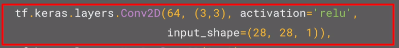
Here we're specifying the first convolution. We're asking keras to generate 64 filters for us. These filters are 3 by 3, their activation is relu, which means the negative values will be thrown away, and finally, the input shape is as before, the 28 by 28. That extra 1 just means that we are tallying using a single byte for color depth. As we saw before our image is our grayscale, so we just use one byte.

Now, of course, you might wonder what the 64 filters are. It's a little beyond the scope of this class to define them, but they aren't random. They start with a set of known good filters in a similar way to the pattern fitting that you saw earlier, and the ones that work from that set are learned over time.

For more details on convolutions and how they work, there's a great set of resources here.

You’ve seen how to add a convolutional 2d layer to the top of your neural network in the previous video. If you want to see more detail on how they worked, check out the playlist at https://bit.ly/2UGa7uH.

Now let’s take a look at adding the pooling, and finishing off the convolutions so you can try them out…

Implementing pooling layers

This next line of code will then create a pooling layer.

It's max-pooling because we're going to take the maximum value. We're saying it's a two-by-two pool, so for every four pixels, the biggest one will survive as shown earlier.

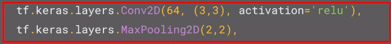
We then add another convolutional layer, and another max-pooling layer so that the network can learn another set of convolutions on top of the existing one, and then again, pool to reduce the size. So, by the time the image gets to the flatten to go into the dense layers, it's already much smaller. It's being quartered, and then quartered again. So, its content has been greatly simplified, the goal being that the convolutions will filter it to the features that determine the output.

A really useful method on the model is the model. summary method.

This allows you to inspect the layers of the model, and see the journey of the image through the convolutions, and here is the output. It's a nice table showing us the layers and some details about them including the output shape.

It's important to keep an eye on the output shape column. When you first look at this, it can be a little bit confusing and feel like a bug. After all, isn't the data 28 by 28, so y is the output, 26 by 26. The key to this is remembering that the filter is a three by three filter. Consider what happens when you start scanning through an image starting on the top left.

So, for example with this image of the dog on the right, you can see zoomed into the pixels at its top left corner. You can't calculate the filter for the pixel in the top left, because it doesn't have any neighbors above it or to its left. In a similar fashion, the next pixel to the right won't work either because it doesn't have any neighbors above it.

So, logically, the first pixel that you can do calculations on is this one, because this one, of course, has all eight neighbors that a three by three filter needs. This when you think about it, means that you can't use a one-pixel margin all around the image, so the output of the convolution will be two pixels smaller on x, and two pixels smaller on y. If your filter is five-by-five for similar reasons, your output will be four smaller on x, and four smaller on y. So, that's y with a three by three filter, our output from the 28 by 28 image, is now 26 by 26, we've removed that one pixel on x and y, and each of the borders. So, next is the first of the max-pooling layers. Now, remember we specified it to be two-by-two, thus turning four pixels into one, and having our x and y.

So, now our output gets reduced from 26 by 26, to 13 by 13. The convolutions will then operate on that, and of course, we lose the one-pixel margin as before, so we're down to 11 by 11, add another two-by-two max-pooling to have this rounding down, and went down, down to five-by-five images. So, now our dense neural network is the same as before, but it's being fed with five-by-five images instead of 28 by 28 ones. But remember, it's not just one compress five-by-five image instead of the original 28 by 28, there are a number of convolutions per image that we specified, in this case, 64. So, there are 64 new images of five-by-five that had been fed in.

Flatten that out and you have 25 pixels times 64, which is 1600. So, you can see that the new flattened layer has 1,600 elements in it, as opposed to the 784 that you had previously. This number is impacted by the parameters that you set when defining the convolutional 2D layers. Later when you experiment, you'll see what the impact of setting what other values for the number of convolutions will be, and in particular, you can see what happens when you're feeding less than 784 overall pixels in. Training should be faster, but is there a sweet spot where it's more accurate? Well, let's switch to the workbook, and we can try it out for ourselves.

Improving the Fashion classifier with convolutions

In the previous video, you looked at convolutions and got a glimpse for how they worked. Bypassing filters over an image to reduce the amount of information, they then allowed the neural network to effectively extract features that can distinguish one class of image from another. You also saw how pooling compresses the information to make it more manageable. This is a really nice way to improve our image recognition performance. Let's now look at it in action using a notebook.

import tensorflow as tf
mnist = tf.keras.datasets.fashion_mnist
(training_images, training_labels), (test_images, test_labels) = mnist.load_data()
training_images=training_images / 255.0
test_images=test_images / 255.0
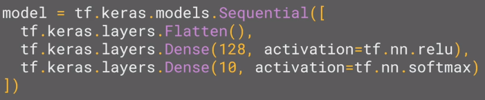
model = tf.keras.models.Sequential([
  tf.keras.layers.Flatten(),
  tf.keras.layers.Dense(128, activation=tf.nn.relu),
  tf.keras.layers.Dense(10, activation=tf.nn.softmax)
])
model.compile(optimizer='adam', loss='sparse_categorical_crossentropy', metrics=['accuracy'])
model.fit(training_images, training_labels, epochs=5)

test_loss = model.evaluate(test_images, test_labels)

Here's the same neural network that you used before for loading the set of images of clothing and then classifying them. By the end of epoch five, you can see the loss is around 0.29, meaning, your accuracy is pretty good on the training data. It took just a few seconds to train, so that's not bad. With the test data as before and as expected, the losses a little higher and thus, the accuracy is a little lower.

Epoch 1/5 60000/60000==============================] - 4s 74us/sample - loss: 0.4989 - acc: 0.8252

Epoch 2/5 60000/60000==============================] - 3s 56us/sample - loss: 0.3745 - acc: 0.8652

Epoch 3/5 60000/60000==============================] - 3s 55us/sample - loss: 0.3378 - acc: 0.8769

Epoch 4/5 60000/60000==============================] - 3s 55us/sample - loss: 0.3126 - acc: 0.8854

Epoch 5/5 60000/60000==============================] - 3s 55us/sample - loss: 0.2943 - acc: 0.8915

10000/10000==============================] - 0s 39us/sample - loss: 0.3594 - acc: 0.8744

Your accuracy is probably about 89% on training and 87% on validation...not bad...But how do you make that even better? One way is to use something called Convolutions. I'm not going to details on Convolutions here, but the ultimate concept is that they narrow down the content of the image to focus on specific, distinct, details.

If you've ever done image processing using a filter (like this: https://en.wikipedia.org/wiki/Kernel_(image_processing)) then convolutions will look very familiar.

In short, you take an array (usually 3x3 or 5x5) and pass it over the image. By changing the underlying pixels based on the formula within that matrix, you can do things like edge detection. So, for example, if you look at the above link, you'll see a 3x3 that is defined for edge detection where the middle cell is 8, and all of its neighbors are -1. In this case, for each pixel, you would multiply its value by 8, then subtract the value of each neighbor. Do this for every pixel, and you'll end up with a new image that has the edges enhanced.

This is perfect for computer vision, because often it's features that can get highlighted like this that distinguish one item for another, and the amount of information needed is then much less...because you'll just train on the highlighted features.

That's the concept of Convolutional Neural Networks. Add some layers to do convolution before you have the dense layers, and then the information going to the dense layers is more focussed, and possibly more accurate.

So now, you can see the code that adds convolutions and pooling. We're going to do two convolutional layers each with 64 convolutions, and each followed by a max pooling layer. You can see that we defined our convolutions to be three-by-three and our pools to be two-by-two. Let's train.

import tensorflow as tf
print(tf.__version__)
mnist = tf.keras.datasets.fashion_mnist
(training_images, training_labels), (test_images, test_labels) = mnist.load_data()
training_images=training_images.reshape(60000, 28, 28, 1)
training_images=training_images / 255.0
test_images = test_images.reshape(10000, 28, 28, 1)
test_images=test_images/255.0
model = tf.keras.models.Sequential([
  tf.keras.layers.Conv2D(64, (3,3), activation='relu', input_shape=(28, 28, 1)),
  tf.keras.layers.MaxPooling2D(2, 2),
  tf.keras.layers.Conv2D(64, (3,3), activation='relu'),
  tf.keras.layers.MaxPooling2D(2,2),
  tf.keras.layers.Flatten(),
  tf.keras.layers.Dense(128, activation='relu'),
  tf.keras.layers.Dense(10, activation='softmax')
])
model.compile(optimizer='adam', loss='sparse_categorical_crossentropy', metrics=['accuracy'])
model.summary()
model.fit(training_images, training_labels, epochs=5)
test_loss = model.evaluate(test_images, test_labels)

The first thing you'll notice is that the training is much slower. For every image, 64 convolutions are being tried, and then the image is compressed and then another 64 convolutions, and then it's compressed again, and then it's passed through the DNN, and that's for 60,000 images that this is happening on each epoch. So it might take a few minutes instead of a few seconds. Now that it's done, you can see that the loss has improved a little.

1.12.0

Epoch 1/5 60000/60000==============================] - 6s 95us/sample - loss: 0.4325 - acc: 0.8411

Epoch 2/5 60000/60000==============================] - 6s 92us/sample - loss: 0.2930 - acc: 0.8914

Epoch 3/5 60000/60000==============================] - 5s 91us/sample - loss: 0.2463 - acc: 0.9079

Epoch 4/5 60000/60000==============================] - 5s 90us/sample - loss: 0.2156 - acc: 0.9187

Epoch 5/5 60000/60000==============================] - 6s 92us/sample - loss: 0.1874 - acc: 0.9307

10000/10000==============================] - 0s 42us/sample - loss: 0.2589 - acc: 0.9089

In this case, it's brought our accuracy up a bit for both our test data and with our training data. That's pretty cool, right? It's likely gone up to about 93% on the training data and 91% on the validation data.

That's significant, and a step in the right direction!

Try running it for more epochs -- say about 20, and explore the results! But while the results might seem really good, the validation results may actually go down, due to something called 'overfitting' which will be discussed later.

(In a nutshell, 'overfitting' occurs when the network learns the data from the training set really well, but it's too specialized to only that data, and as a result, is less effective at seeing other data. For example, if all your life you only saw red shoes, then when you see a red shoe you would be very good at identifying it, but blue suede shoes might confuse you...and you know you should never mess with my blue suede shoes.)

Then, look at the code again, and see, step by step how the Convolutions were built:

Step 1 is to gather the data. You'll notice that there's a bit of a change here in that the training data needed to be reshaped. That's because the first convolution expects a single tensor containing everything, so instead of 60,000 28x28x1 items in a list, we have a single 4D list that is 60,000x28x28x1, and the same for the test images. If you don't do this, you'll get an error when training as the Convolutions do not recognize the shape.

import tensorflow as tf
mnist = tf.keras.datasets.fashion_mnist
(training_images, training_labels), (test_images, test_labels) = mnist.load_data()
training_images=training_images.reshape(60000, 28, 28, 1)
training_images=training_images / 255.0
test_images = test_images.reshape(10000, 28, 28, 1)
test_images=test_images/255.0

Next is to define your model. Now instead of the input layer at the top, you're going to add a Convolution. The parameters are:

The number of convolutions you want to generate. Purely arbitrary, but good to start with something in the order of 32
The size of the Convolution, in this case, a 3x3 grid
The activation function to use -- in this case we'll use relu, which you might recall is the equivalent of returning x when x>0, else return 0
In the first layer, the shape of the input data.

You'll follow the Convolution with a MaxPooling layer which is then designed to compress the image while maintaining the content of the features that were highlighted by the convolution. By specifying (2,2) for the MaxPooling, the effect is to quarter the size of the image. Without going into too much detail here, the idea is that it creates a 2x2 array of pixels, and picks the biggest one, thus turning 4 pixels into 1. It repeats this across the image, and in so doing halves the number of horizontal, and halves the number of vertical pixels, effectively reducing the image by 25%.

You can call model.summary() to see the size and shape of the network, and you'll notice that after every MaxPooling layer, the image size is reduced in this way.

model = tf.keras.models.Sequential([
  tf.keras.layers.Conv2D(32, (3,3), activation='relu', input_shape=(28, 28, 1)),
  tf.keras.layers.MaxPooling2D(2, 2),

Add another convolution

  tf.keras.layers.Conv2D(64, (3,3), activation='relu'),
  tf.keras.layers.MaxPooling2D(2,2)

Now flatten the output. After this, you'll just have the same DNN structure as the non-convolutional version

  tf.keras.layers.Flatten(),

The same 128 dense layers, and 10 output layers as in the pre-convolution example:

  tf.keras.layers.Dense(128, activation='relu'),
  tf.keras.layers.Dense(10, activation='softmax')
])

Now compile the model, call the fit method to do the training, and evaluate the loss and accuracy from the test set.

model.compile(optimizer='adam', loss='sparse_categorical_crossentropy', metrics=['accuracy'])
model.fit(training_images, training_labels, epochs=5)
test_loss, test_acc = model.evaluate(test_images, test_labels)
print(test_acc)

Now, let's take a look at the code at the bottom of the notebook. Now, this is a really fun visualization of the journey of an image through the convolutions.

Visualizing the Convolutions and Pooling

This code will show us the convolutions graphically. The print (test_labels[;100]) shows us the first 100 labels in the test set, and you can see that the ones at index 0, index 23 and index 28 are all the same value (9). They're all shoes. Let's take a look at the result of running the convolution on each, and you'll begin to see common features between them emerge. Now, when the DNN is training on that data, it's working with a lot less, and it's perhaps finding a commonality between shoes based on this convolution/pooling combination.

print(test_labels[:100])

First, I'll print out the first 100 test labels. The number nine as we saw earlier is a shoe or boots. I picked out a few instances of this whether the zero, the 23rd and the 28th labels are all nine. So let's take a look at their journey.

[9 2 1 1 6 1 4 6 5 7 4 5 7 3 4 1 2 4 8 0 2 5 7 9 1 4 6 0 9 3 8 8 3 3 8 0 7 5 7 9 6 1 3 7 6 7 2 1 2 2 4 4 5 8 2 2 8 4 8 0 7 7 8 5 1 1 2 3 9 8 7 0 2 6 2 3 1 2 8 4 1 8 5 9 5 0 3 2 0 6 5 3 6 7 1 8 0 1 4 2]

The Keras API gives us each convolution and each pooling and each dense, etc. as a layer. So with the layers API, I can take a look at each layer's outputs, so I'll create a list of each layer's output. I can then treat each item in the layer as an individual activation model if I want to see the results of just that layer.

Now, by looping through the layers, I can display the journey of the image through the first convolution and then the first pooling and then the second convolution and then the second pooling. Note how the size of the image is changing by looking at the axes. If I set the convolution number to one, we can see that it almost immediately detects the laces area as a common feature between the shoes.

import matplotlib.pyplot as plt
f, axarr = plt.subplots(3,4)
FIRST_IMAGE=0
SECOND_IMAGE=7
THIRD_IMAGE=26
CONVOLUTION_NUMBER = 1
from tensorflow.keras import models
layer_outputs = [layer.output for layer in model.layers]
activation_model = tf.keras.models.Model(inputs = model.input, outputs = layer_outputs)
for x in range(0,4):
  f1 = activation_model.predict(test_images[FIRST_IMAGE].reshape(1, 28, 28, 1))[x]
  axarr[0,x].imshow(f1[0, : , :, CONVOLUTION_NUMBER], cmap='inferno')
  axarr[0,x].grid(False)
  f2 = activation_model.predict(test_images[SECOND_IMAGE].reshape(1, 28, 28, 1))[x]
  axarr[1,x].imshow(f2[0, : , :, CONVOLUTION_NUMBER], cmap='inferno')
  axarr[1,x].grid(False)
  f3 = activation_model.predict(test_images[THIRD_IMAGE].reshape(1, 28, 28, 1))[x]
  axarr[2,x].imshow(f3[0, : , :, CONVOLUTION_NUMBER], cmap='inferno')
  axarr[2,x].grid(False)

So, for example, if I change the third image to be one, which looks like a handbag, you'll see that it also has a bright line near the bottom that could look like the soul of the shoes, but by the time it gets through the convolutions, that's lost, and that area for the laces doesn't even show up at all.

So this convolution definitely helps me separate issue from a handbag. Again, if I said it's a two, it appears to be trousers, but the feature that detected something that the shoes had in common fails again. Also, if I changed my third image back to that for the shoe, but I tried a different convolution number, you'll see that for convolution two, it didn't really find any common features. To see the commonality in a different image, try images two, three, and five. These all appear to be trousers. Convolutions two and four seem to detect this vertical feature as something they all have in common. If I again go to the list and find three labels that are the same, in this case, six, I can see what they signify. When I run it, I can see that they appear to be shirts. Convolution four doesn't do a whole lot, so let's try five. We can kind of see that the color appears to light up in this case. Let's try convolution one. I don't know about you, but I can play with this all day. Then see what you do when you run it for yourself. When you're done playing, try tweaking the code with these suggestions, editing the convolutions, removing the final convolution, and adding more, etc.

Also, in a previous exercise, you added a callback that finished training once the loss had a certain amount. So try to add that here. When you're done, we'll move to the next stage, and that's dealing with images that are larger and more complex than these ones. To see how convolutions can maybe detect features when they aren't always in the same place like they would be in these tightly controlled 28 by 28 images.

Here’s the notebook that Laurence was using in that screencast. To make it work quicker, go to the ‘Runtime’ menu, and select ‘Change runtime type’. Then select GPU as the hardware accelerator!

Work through it, and try some of the exercises at the bottom! It's really worth spending a bit of time on these because, as before, they'll really help you by seeing the impact of small changes to various parameters in the code. You should spend at least 1 hour on this today!

Once you’re done, go onto the next video and take a look at some code to build a convolution yourself to visualize how it works!

EXERCISES

Try editing the convolutions. Change the 32s to either 16 or 64. What impact will this have on accuracy and/or training time?
Remove the final Convolution. What impact will this have on accuracy or training time?
How about adding more Convolutions? What impact do you think this will have? Experiment with it.
Remove all Convolutions but the first. What impact do you think this will have? Experiment with it.
In the previous lesson, you implemented a callback to check on the loss function and to cancel training once it hit a certain amount. See if you can implement that here!

import tensorflow as tf
print(tf.__version__)
mnist = tf.keras.datasets.mnist
(training_images, training_labels), (test_images, test_labels) = mnist.load_data()
training_images=training_images.reshape(60000, 28, 28, 1)
training_images=training_images / 255.0
test_images = test_images.reshape(10000, 28, 28, 1)
test_images=test_images/255.0
model = tf.keras.models.Sequential([
  tf.keras.layers.Conv2D(32, (3,3), activation='relu', input_shape=(28, 28, 1)),
  tf.keras.layers.MaxPooling2D(2, 2),
  tf.keras.layers.Flatten(),
  tf.keras.layers.Dense(128, activation='relu'),
  tf.keras.layers.Dense(10, activation='softmax')
])
model.compile(optimizer='adam', loss='sparse_categorical_crossentropy', metrics=['accuracy'])
model.fit(training_images, training_labels, epochs=10)
test_loss, test_acc = model.evaluate(test_images, test_labels)
print(test_acc)

1.12.0

Epoch 1/10 60000/60000==============================] - 6s 104us/sample - loss: 0.1510 - acc: 0.9551

Epoch 2/10 60000/60000==============================] - 5s 79us/sample - loss: 0.0512 - acc: 0.9843

Epoch 3/10 60000/60000==============================] - 5s 77us/sample - loss: 0.0319 - acc: 0.9902

Epoch 4/10 60000/60000==============================] - 5s 78us/sample - loss: 0.0209 - acc: 0.9934

Epoch 5/10 60000/60000==============================] - 5s 78us/sample - loss: 0.0136 - acc: 0.9956

Epoch 6/10 60000/60000==============================] - 5s 78us/sample - loss: 0.0111 - acc: 0.9964

Epoch 7/10 60000/60000==============================] - 5s 79us/sample - loss: 0.0076 - acc: 0.9974

Epoch 8/10 60000/60000==============================] - 5s 78us/sample - loss: 0.0052 - acc: 0.9985

Epoch 9/10 60000/60000==============================] - 5s 81us/sample - loss: 0.0046 - acc: 0.9988

Epoch 10/10 60000/60000==============================] - 5s 81us/sample - loss: 0.0053 - acc: 0.9981

10000/10000==============================] - 1s 53us/sample - loss: 0.0583 - acc: 0.9873 0.9873

Walking through convolutions

In the previous lessons, you saw the impacts that convolutions and pooling had on your networks efficiency and learning, but a lot of that was theoretical in nature. So I thought it'd be interesting to hack some code together to show how a convolution actually works. We'll also create a little pooling algorithm, so you can visualize its impact.

There's a notebook that you can play with too, and I'll step through that here. Here's the notebook for playing with convolutions. It does use a few Python libraries that you may not be familiar with such as cv2. It also has Matplotlib that we used before. If you haven't used them, they're really quite intuitive for this task and they're very very easy to learn. So first, we'll set up our inputs and in particular, import the misc library from SciPy. Now, this is a nice shortcut for us because misc.ascent returns a nice image that we can play with, and we don't have to worry about managing our own. Matplotlib contains the code for drawing an image and it will render it right in the browser with Colab. Here, we can see the ascent image from SciPy.

import cv2
import numpy as np
from scipy import misc
i = misc.ascent()


import matplotlib.pyplot as plt
plt.grid(False)
plt.gray()
plt.axis('off')
plt.imshow(i)
plt.show()

The image is stored as a numpy array, so we can create the transformed image by just copying that array. Let's also get the dimensions of the image so we can loop over it later.

i_transformed = np.copy(i)
size_x = i_transformed.shape[0]
size_y = i_transformed.shape[1]

Now we can create a filter as a 3x3 array. Next up, we'll take a copy of the image, and we'll add it with our homemade convolutions, and we'll create variables to keep track of the x and y dimensions of the image. So we can see here that it's a 512 by 512 image.

# This filter detects edges nicely
# It creates a convolution that only passes through sharp edges and straight
# lines.

#Experiment with different values for fun effects.
#filter = [ [0, 1, 0], [1, -4, 1], [0, 1, 0]]

# A couple more filters to try for fun!
filter = [ [-1, -2, -1], [0, 0, 0], [1, 2, 1]]
#filter = [ [-1, 0, 1], [-2, 0, 2], [-1, 0, 1]]

# If all the digits in the filter don't add up to 0 or 1, you 
# should probably do a weight to get it to do so
# so, for example, if your weights are 1,1,1 1,2,1 1,1,1
# They add up to 10, so you would set a weight of .1 if you want to normalize them
weight  = 1

Now let's create a convolution. We will iterate over the image, leaving a 1-pixel margin, and multiply out each of the neighbors of the current pixel by the value defined in the filter.

i.e. the current pixel's neighbor above it and to the left will be multiplied by the top left item in the filter etc. etc. We'll then multiply the result by the weight, and then ensure the result is in the range 0-255

Finally, we'll load the new value into the transformed image.

for x in range(1,size_x-1):
  for y in range(1,size_y-1):
      convolution = 0.0
      convolution = convolution + (i[x - 1, y-1] * filter[0][0])
      convolution = convolution + (i[x, y-1] * filter[0][1])
      convolution = convolution + (i[x + 1, y-1] * filter[0][2])
      convolution = convolution + (i[x-1, y] * filter[1][0])
      convolution = convolution + (i[x, y] * filter[1][1])
      convolution = convolution + (i[x+1, y] * filter[1][2])
      convolution = convolution + (i[x-1, y+1] * filter[2][0])
      convolution = convolution + (i[x, y+1] * filter[2][1])
      convolution = convolution + (i[x+1, y+1] * filter[2][2])
      convolution = convolution * weight
      if(convolution<0):
        convolution=0
      if(convolution>255):
        convolution=255
      i_transformed[x, y] = convolution

So now, let's create a convolution as a three by three array. We'll load it with values that are pretty good for detecting sharp edges first. Here's where we'll create the convolution. We iterate over the image, leaving a one-pixel margin. You'll see that the loop starts at one and not zero, and it ends at size x minus one and size y minus one. In the loop, it will then calculate the convolution value by looking at the pixel and its neighbors, and then by multiplying them out by the values determined by the filter, before finally summing it all up. Let's run it. It takes just a few seconds, so when it's done, let's draw the results. We can see that only certain features made it through the filter.

# Plot the image. Note the size of the axes -- they are 512 by 512
plt.gray()
plt.grid(False)
plt.imshow(i_transformed)
#plt.axis('off')
plt.show()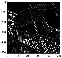

I've provided a couple more filters, so let's try them. This first one is really great at spotting vertical lines. So when I run it and plot the results, we can see that the vertical lines in the image made it through. It's really cool because they're not just straight up and down, they are vertical in perspective within the perspective of the image itself. Similarly, this filter works well for horizontal lines. So when I run it, and then plot the results, we can see that a lot of the horizontal lines made it through.

Now, let's take a look at pooling, and in this case, Max pooling, which takes pixels in chunks of four and only passes through the biggest value. This code will show a (2, 2) pooling. The idea here is to iterate over the image and look at the pixel and it's immediate neighbors to the right, beneath, and right-beneath. Take the largest of them and load it into the new image. Thus the new image will be 1/4 the size of the old -- with the dimensions on X and Y being halved by this process. You'll see that the features get maintained despite this compression!

new_x = int(size_x/2)
new_y = int(size_y/2)
newImage = np.zeros((new_x, new_y))
for x in range(0, size_x, 2):
  for y in range(0, size_y, 2):
    pixels = []
    pixels.append(i_transformed[x, y])
    pixels.append(i_transformed[x+1, y])
    pixels.append(i_transformed[x, y+1])
    pixels.append(i_transformed[x+1, y+1])
    pixels.sort(reverse=True)
    newImage[int(x/2),int(y/2)] = pixels[0]

# Plot the image. Note the size of the axes -- now 256 pixels instead of 512
plt.gray()
plt.grid(False)
plt.imshow(newImage)
#plt.axis('off')
plt.show()

I run the code and then render the output. We can see that the features of the image are maintained, but look closely at the axes, and we can see that the size has been halved from the 500's to the 250's. For fun, we can try the other filter, run it, and then compare the convolution with its pooled version. Again, we can see that the features have not just been maintained, they may have also been emphasized a bit.

So that's how convolutions work. Under the hood, TensorFlow is trying different filters on your image and learning which ones work when looking at the training data. As a result, when it works, you'll have greatly reduced information passing through the network, but because it isolates and identifies features, you can also get increased accuracy. Have a play with the filters in this workbook and see if you can come up with some interesting effects of your own.

To try this notebook for yourself, and play with some convolutions, here’s the notebook. Let us know if you come up with any interesting filters of your own!

As before, spend a little time playing with this notebook. Try different filters, and research different filter types. There's some fun information about them here: https://lodev.org/cgtutor/filtering.html

This course uses a third-party tool, Exercise 3 - Improve MNIST with convolutions, to enhance your learning experience. No personal information will be shared with the tool.

import tensorflow as tf

class myCallback(tf.keras.callbacks.Callback):
  def on_epoch_end(self, epoch, logs={}):
    if(logs.get('acc')>0.998):
      print("\nReached 99.8% accuracy so cancelling training!")
      self.model.stop_training = True

callbacks = myCallback()
mnist = tf.keras.datasets.mnist
(training_images, training_labels), (test_images, test_labels) = mnist.load_data()
training_images=training_images.reshape(60000, 28, 28, 1)
training_images=training_images / 255.0
test_images = test_images.reshape(10000, 28, 28, 1)
test_images=test_images/255.0
model = tf.keras.models.Sequential([
  tf.keras.layers.Conv2D(32, (3,3), activation='relu', input_shape=(28, 28, 1)),
  tf.keras.layers.MaxPooling2D(2, 2),
  tf.keras.layers.Flatten(),
  tf.keras.layers.Dense(128, activation='relu'),
  tf.keras.layers.Dense(10, activation='softmax')
])
model.compile(optimizer='adam', loss='sparse_categorical_crossentropy', metrics=['accuracy'])
model.fit(training_images, training_labels, epochs=10, callbacks=[callbacks])

[Introduction to TensorFlow] Enhancing Vision with Convolutional Neural Networks(Video & Exercise)