As Andrew and Laurence discussed, the techniques you’ve learned already can apply to complex images, and you can start solving real scenarios with them. They discussed how it could be used, for example, in disease detection with the Cassava plant, and you can see a video demonstrating that TensorFlow: an ML platform for solving impactful and challenging problems. Once you’ve watched that, move onto the next lesson!
You used a few notebooks this week. For your convenience, or offline use, I've shared them on GitHub. The links are below:
Horses or Humans with Validation
Horses or Humans with Compacting of Images
Understanding ImageGenerator
To this point, you built an image classifier that worked using a deep neural network and you saw how to improve its performance by adding convolutions. One limitation though was that it used a dataset of very uniform images. Images of clothing that was staged and framed in 28 by 28. But what happens when you use larger images and where the feature might be in different locations?

For example, how about these images of horses and humans? They have different sizes and different aspect ratios. The subject can be in different locations. In some cases, there may even be multiple subjects. In addition to that, the earlier examples with fashion data used a built-in dataset. All of the data was handily split into training and test sets for you and labels were available.
In many scenarios, that's not going to be the case and you'll have to do it for yourself. So in this lesson, we'll take a look at some of the APIs that are available to make that easier for you. In particular, the image generator in TensorFlow.
One feature of the image generator is that you can point it at a directory and then the sub-directories of that will automatically generate labels for you.

So for example, consider this directory structure. You have an images directory and in that, you have sub-directories for training and validation. When you put sub-directories in these for horses and humans and store the requisite images in there, the image generator can create a feeder for those images and auto label them for you.
So for example, if I point an image generator at the training directory, the labels will be horses and humans and all of the images in each directory will be loaded and labeled accordingly. Similarly, if I point one at the validation directory, the same thing will happen.
So let's take a look at this in code.
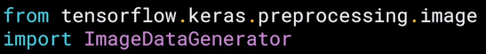
The image generator class is available in Keras.preprocessing.image. You can then instantiate an image generator like this.
I'm going to pass rescale to it to normalize the data.

You can then call the flow from directory method on it to get it to load images from that directory and its sub-directories. It's a common mistake that people point the generator at the sub-directory. It will fail in that circumstance. You should always point it at the directory that contains sub-directories that contain your images. The names of the sub-directories will be the labels for your images that are contained within them. So make sure that the directory you're pointing to is the correct one. You put it in the second parameter like this. Now, images might come in all shapes and sizes and unfortunately for training a neural network, the input data all has to be the same size, so the images will need to be resized to make them consistent.
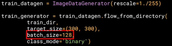
The nice thing about this code is that the images are resized for you as they're loaded. So you don't need to preprocess thousands of images on your file system. But you could have done that if you wanted to. The advantage of doing it at runtime like this is that you can then experiment with different sizes without impacting your source data. While the horses and humans dataset is already in 300 by 300, when you use other datasets they may not always be uniformly sized. So this is really useful for you. The images will be loaded for training and validation in batches where it's more efficient than doing it one by one. Now, there's a whole science to calculating batch size that's beyond the scope of this course, but you can experiment with different sizes to see the impact on the performance by changing this parameter.
Finally, there's the class mode. Now, this is a binary classifier i.e. it picks between two different things; horses and humans, so we specify that here. Other options in particular for more than two things will be explored later in the course.

The validation generator should be exactly the same except of course it points at a different directory, the one containing the sub-directories containing the test images.
When you go through the workbook shortly, you'll see how to download the images as a zip, and then sort them into training and test sub-directories, and then put horses and humans sub-directories in each. That's just pure Python. It's not TensorFlow or any other deep learning stuff. But it's all explained for you in the notebook.
Defining a ConvNet to use complex images
So let's now take a look at the definition of the neural network that we'll use to classify horses versus humans. It's very similar to what you just used for the fashion items, but there are a few minor differences based on this data and the fact that we're using generators.
So here's the code.

As you can see, it's sequential as before with convolutions and pooling before we get to the dense layers at the bottom. But let's highlight some of the differences. First of all, you'll notice that there are three sets of convolution pooling layers at the top. This reflects the higher complexity and size of the images. Remember our earlier our 28 by 28.5 to 13 and then five before flattening, well, now we have 300 by 300. So we start at 298 by 298 and then have that etc., etc. until, by the end, we're at a 35 by 35 image. We can even add another couple of layers to this if we wanted to get to the same ballpark size as previously, but we'll keep it at three for now.

Another thing to pay attention to is the input shape. We resize their images to be 300 by 300 as they were loaded, but they're also color images. So there are three bytes per pixel. One byte for the red, one for green, and one for the blue channel, and that's a common 24-bit color pattern.
![]()
If you're paying really close attention, you can see that the output layer has also changed. Remember before when you created the output layer, you had one neuron per class, but now there's only one neuron for two classes. That's because we're using a different activation function where sigmoid is great for binary classification, where one class will tend towards zero and the other class tending towards one. You could use two neurons here if you want, and the same softmax function as before, but for binary, this is a bit more efficient.
If you want you can experiment with the workbook and give it a try yourself.

Now, if we take a look at our model summary, we can see the journey of the image data through the convolutions The 300 by 300 becomes 298 by 298 after the three by three filter, it gets pulled to 149 by 149 which in turn gets reduced to 73 by 73 after the filter that then gets pulled to 35 by 35, this will then get flattened, so 64 convolutions that are 35 squared and shape will get fed into the DNN. If you multiply 35 by 35 by 64, you get 78,400, and that's the shape of the data once it comes out of the convolutions. If we had just fed raw 300 by 300 images without the convolutions, that would be over 900,000 values. So we've already reduced it quite a bit.
Training the ConvNet with fit_generator
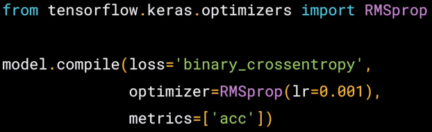
Okay, we'll now compile the model and, as always, we have a loss function and an optimizer. When classifying the ten items of fashion, you might remember that your loss function was a categorical cross entropy. But because we're doing a binary choice here, let's pick a binary_crossentropy instead. Also, earlier we used an Adam optimizer. Now, you could do that again, but I thought it would be fun to use the RMSprop, where you can adjust the learning rate to experiment with performance.
To understand the learning rate and how all that fits together, check out this great video from deeplearning.ai that goes into it in a lot more detail.
For now, I'm not going to go into the details in this course. Okay, next up is the training, now, this looks a little different than before when you called model.fit.

Because now you call model.fit_generator, and that's because we're using a generator instead of datasets. Remember the image generator from earlier, let's look at each parameter in detail.
The first parameter is the training generator that you set up earlier. This streams the images from the training directory. Remember the batch size you used when you created it, it was 20, that's important in the next step.
There are 1,024 images in the training directory, so we're loading them in 128 at a time. So in order to load them all, we need to do 8 batches. So we set the steps_per_epoch to cover that.
Here we just set the number of epochs to train for. This is a bit more complex, so let's use, say, 15 epochs in this case.
And now we specify the validation set that comes from the validation_generator that we also created earlier.
It had 256 images, and we wanted to handle them in batches of 32, so we will do 8 steps.

And the verbose parameter specifies how much to display while training is going on. With verbose set to 2, we'll get a little less animation hiding the epoch progress.
Once the model is trained, you will, of course, want to do some prediction on the model. And here's the code to do that, let's look at it piece by piece.

So these parts are specific to Colab, they are what gives you the button that you can press to pick one or more images to upload. The image paths then get loaded into this list called uploading. The loop then iterates through all of the images in that collection. And you can load an image and prepare it to input into the model with this code.
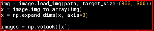
Take note to ensure that the dimensions match the input dimensions that you specified when designing the model. You can then call the model. predict, passing it the details, and it will return an array of classes. In the case of binary classification, this will only contain one item with a value close to 0 for one class and close to 1 for the other.
Later in this course, you'll see multi-class classification with Softmax. Where you'll get a list of values with one value for the probability of each class and all of the probabilities adding up to 1.
Walking through developing a ConvNet
Okay. So you've just seen how to get started with creating a neural network in Keras that uses the image generator to automatically load and label your files based on their subdirectories. Now, let's see how we can use that to build horses or humans classifier with a convolutional neural network.
This is the first notebook you can try. To start, you'll download the zip file containing the horses and humans data.
import os
import zipfile

local_zip = '/tmp/horse-or-human.zip'
zip_ref = zipfile.ZipFile(local_zip, 'r')
zip_ref.extractall('/tmp/horse-or-human')
zip_ref.close()
Once that's done, you can unzip it to the temp directory on this virtual machine.
The contents of the .zip are extracted to the base directory, /tmp/horse-or-human which in turn each contain horses and humans subdirectories. In short: The training set is the data that is used to tell the neural network model that 'this is what a horse looks like', 'this is what a human looks like' etc. One thing to pay attention to in this sample: We do not explicitly label the images as horses or humans. If you remember with the handwriting example earlier, we had labeled 'this is a 1', 'this is a 7' etc. Later you'll see something called an ImageGenerator being used -- and this is coded to read images from subdirectories, and automatically label them from the name of that subdirectory. So, for example, you will have a 'training' directory containing a 'horses' directory and a 'humans' one. ImageGenerator will label the images appropriately for you, reducing a coding step.
Let's define each of these directories: The zip file contains two folders; one called filtered horses, and one called filtered humans. When it was unzipped, these were created for you.
# Directory with our training horse pictures
train_horse_dir = os.path.join('/tmp/horse-or-human/horses')

# Directory with our training human pictures
train_human_dir = os.path.join('/tmp/horse-or-human/humans')
So we'll just point a couple of variables at them, and then we can explore the files by printing out some of the filenames. Now, these could be used to generate labels, but we won't need that if we use the Keras generator. If you wanted to use this data without one, filenames will have the labels in them of course though.
train_horse_names = os.listdir(train_horse_dir)
print(train_horse_names[:10])

train_human_names = os.listdir(train_human_dir)
print(train_human_names[:10])
['horse01-0.png', 'horse01-1.png', 'horse01-2.png', 'horse01-3.png', 'horse01-4.png', 'horse01-5.png', 'horse01-6.png', 'horse01-7.png', 'horse01-8.png', 'horse01-9.png'] ['human01-00.png', 'human01-01.png', 'human01-02.png', 'human01-03.png', 'human01-04.png', 'human01-05.png', 'human01-06.png', 'human01-07.png', 'human01-08.png', 'human01-09.png']
We'll print out the number of images that we have to work with, and there's a little over 1000 of them, and now we can display a few random images from the dataset.
print('total training horse images:', len(os.listdir(train_horse_dir)))
print('total training human images:', len(os.listdir(train_human_dir)))
total training horse images: 500 total training human images: 527
%matplotlib inline

import matplotlib.pyplot as plt
import matplotlib.image as mpimg

# Parameters for our graph; we'll output images in a 4x4 configuration
nrows = 4
ncols = 4

# Index for iterating over images
pic_index = 0
# Set up matplotlib fig, and size it to fit 4x4 pics
fig = plt.gcf()
fig.set_size_inches(ncols * 4, nrows * 4)
pic_index += 8
next_horse_pix = [os.path.join(train_horse_dir, fname)
for fname in train_horse_names[pic_index-8:pic_index]]
next_human_pix = [os.path.join(train_human_dir, fname)
for fname in train_human_names[pic_index-8:pic_index]]
for i, img_path in enumerate(next_horse_pix+next_human_pix):
# Set up subplot; subplot indices start at 1
sp = plt.subplot(nrows, ncols, i + 1)
sp.axis('Off') # Don't show axes (or gridlines)
img = mpimg.imread(img_path)
plt.imshow(img)
plt.show()Here, we can see eight horses and eight humans.

An interesting aspect of this dataset is that all of the images are computer-generated. I've rendered them to be as photo-real as possible, but there'll be actually used to classify real pictures of horses and people, and here are a few more images just to show some of the diversity.
Building a Small Model from Scratch
Let's start building the model.
First, we'll import TensorFlow, and now we'll build the layers. We have quite a few convolutions here because our source images are quite large, are 300 by 300.
model = tf.keras.models.Sequential([
# Note the input shape is the desired size of the image 300x300 with 3 bytes color
# This is the first convolution
tf.keras.layers.Conv2D(16, (3,3), activation='relu', input_shape=(300, 300, 3)),
tf.keras.layers.MaxPooling2D(2, 2),
# The second convolution
tf.keras.layers.Conv2D(32, (3,3), activation='relu'),
tf.keras.layers.MaxPooling2D(2,2),
# The third convolution
tf.keras.layers.Conv2D(64, (3,3), activation='relu'),
tf.keras.layers.MaxPooling2D(2,2),
# The fourth convolution
tf.keras.layers.Conv2D(64, (3,3), activation='relu'),
tf.keras.layers.MaxPooling2D(2,2),
# The fifth convolution
tf.keras.layers.Conv2D(64, (3,3), activation='relu'),
tf.keras.layers.MaxPooling2D(2,2),
# Flatten the results to feed into a DNN
tf.keras.layers.Flatten(),
# 512 neuron hidden layer
tf.keras.layers.Dense(512, activation='relu'),
# Only 1 output neuron. It will contain a value from 0-1 where 0 for 1 class ('horses') and 1 for the other ('humans')
tf.keras.layers.Dense(1, activation='sigmoid')
])Later we can explore the impact of reducing their size and needing fewer convolutions. We can print the summary of the layers, and here we can see by the time we reach the dense network, the convolutions are down to seven-by-seven.
model.summary()
Okay. Next up, we'll compiler network. It's using binary cross-entropy as the loss, binary because we're using just two classes, and the optimizer is an RMSprop that allows us to tweak the learning rate. Don't worry if you don't fully understand these yet, there are links out to content about them where you can learn more.
from tensorflow.keras.optimizers import RMSprop
model.compile(loss='binary_crossentropy',
optimizer=RMSprop(lr=0.001),
metrics=['acc'])Now that you’ve learned how to download and process the horses and humans dataset, you’re ready to train. When you defined the model, you saw that you were using a new loss function called ‘Binary Cross-entropy’, and a new optimizer called RMSProp. If you want to learn more about the type of binary classification we are doing here, check out this great video from Andrew!


Walking through training the ConvNet with fit_generator(Training)
Next up is where we use the ImageDataGenerator. We instantiate it and we scale our images to 1 over 255, which then normalizes their values. We then point it at the main directory where we see the unzipped files.
As you may already know, data that goes into neural networks should usually be normalized in some way to make it more amenable to processing by the network. (It is uncommon to feed raw pixels into a convnet.) In our case, we will preprocess our images by normalizing the pixel values to be in the [0, 1] range (originally all values are in the [0, 255] range).
In Keras this can be done via the keras.preprocessing.image.ImageDataGenerator class using the rescale parameter. This ImageDataGenerator class allows you to instantiate generators of augmented image batches (and their labels) via .flow(data, labels) or .flow_from_directory(directory). These generators can then be used with the Keras model methods that accept data generators as inputs: fit_generator, evaluate_generator, and predict_generator.
from tensorflow.keras.preprocessing.image import ImageDataGenerator
# All images will be rescaled by 1./255
train_datagen = ImageDataGenerator(rescale=1/255)
# Flow training images in batches of 128 using train_datagen generator
train_generator = train_datagen.flow_from_directory(
'/tmp/horse-or-human/', # This is the source directory for training images
target_size=(300, 300), # All images will be resized to 150x150
batch_size=128,
# Since we use binary_crossentropy loss, we need binary labels
class_mode='binary')
We can see that it finds all of the images, and has assigned them to two classes because they were two subdirectories. We'll now train the neural network for 15 epochs, it will take about two minutes.
history = model.fit_generator(
train_generator,
steps_per_epoch=8,
epochs=15,
verbose=1)
Each epoch is loading the data, calculating the convolutions and then trying to match the convolutions to labels. As you can see, the accuracy mostly increases but it will occasionally deep, showing the gradient ascent of the learning actually in action. It's always a good idea to keep an eye on fluctuations in this figure. And if there are too wild, you can adjust the learning rate. Remember the parameter to RMS prop when you compile the model, that's where you'd tweak it. It's also going pretty fast, because right here, I'm training on a GPU machine. By the time we get to epoch 15, we can see that our accuracy is about 0.9981, which is really good. But remember, that's only based on the data that the network has already seen during training, which is only about 1,000 images. So don't get lulled into a false sense of security.
Let's have a bit of fun with the model now and see if we can predict the class for new images that it hasn't previously seen.
Running the Model
Let's now take a look at actually running a prediction using the model. This code will allow you to choose 1 or more files from your file system, it will then upload them, and run them through the model, giving an indication of whether the object is a horse or a human.
import numpy as np
from google.colab import files
from keras.preprocessing import image
uploaded = files.upload()
for fn in uploaded.keys():
# predicting images
path = '/content/' + fn
img = image.load_img(path, target_size=(300, 300))
x = image.img_to_array(img)
x = np.expand_dims(x, axis=0)
images = np.vstack([x])
classes = model.predict(images, batch_size=10)
print(classes[0])
if classes[0]>0.5:
print(fn + " is a human")
else:
print(fn + " is a horse")
Let's go to Pixabay, and see what we can find. I'll search for horses, and there's lots of horses, so let's pick this one. It's a white horse running in the snow. I'm going to download it to my file system. I'm now going to go back to the notebook, and I'm going to upload the image from my file system.
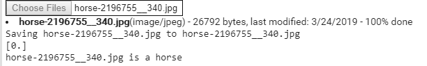
And we'll see that it gets uploaded, and it's classified as a horse. So let's try another one. Like this one here. Which I'll then upload to the notebook, and we'll see that it's also classified as a horse. I'll now go back to Pixabay and search for a person, and pick this image of a girl sitting on a bench. I'll download it to my file system, upload it to the neural network, and we can see that this is also correctly classified as a human.
Let's do one more. I'll go back to the list of results on Pixabay, and pick this image of a girl. As before, I'll download it to my file system and I'll upload it to the neural network and we'll also see that it's still detects a human in the image. Now one other thing that I can do with this script is uploaded multiple files and have it classify all of them at once. And here we can see all of the classifications. We have four out four correct. This notebook also includes some visualizations of the image as it passes through the convolutions. You can give it a try with this script. Here you can see where a human image was convolved and features such as the legs really lit up.
import numpy as np
import random
from tensorflow.keras.preprocessing.image import img_to_array, load_img
# Let's define a new Model that will take an image as input, and will output
# intermediate representations for all layers in the previous model after
# the first.
successive_outputs = [layer.output for layer in model.layers[1:]]
#visualization_model = Model(img_input, successive_outputs)
visualization_model = tf.keras.models.Model(inputs = model.input, outputs = successive_outputs)
# Let's prepare a random input image from the training set.
horse_img_files = [os.path.join(train_horse_dir, f) for f in train_horse_names]
human_img_files = [os.path.join(train_human_dir, f) for f in train_human_names]
img_path = random.choice(horse_img_files + human_img_files)
img = load_img(img_path, target_size=(300, 300)) # this is a PIL image
x = img_to_array(img) # Numpy array with shape (150, 150, 3)
x = x.reshape((1,) + x.shape) # Numpy array with shape (1, 150, 150, 3)
# Rescale by 1/255
x /= 255
# Let's run our image through our network, thus obtaining all
# intermediate representations for this image.
successive_feature_maps = visualization_model.predict(x)
# These are the names of the layers, so can have them as part of our plot
layer_names = [layer.name for layer in model.layers]
# Now let's display our representations
for layer_name, feature_map in zip(layer_names, successive_feature_maps):
if len(feature_map.shape) == 4:
# Just do this for the conv / maxpool layers, not the fully-connected layers
n_features = feature_map.shape[-1] # number of features in feature map
# The feature map has shape (1, size, size, n_features)
size = feature_map.shape[1]
# We will tile our images in this matrix
display_grid = np.zeros((size, size * n_features))
for i in range(n_features):
# Postprocess the feature to make it visually palatable
x = feature_map[0, :, :, i]
x -= x.mean()
x /= x.std()
x *= 64
x += 128
x = np.clip(x, 0, 255).astype('uint8')
# We'll tile each filter into this big horizontal grid
display_grid[:, i * size : (i + 1) * size] = x
# Display the grid
scale = 20. / n_features
plt.figure(figsize=(scale * n_features, scale))
plt.title(layer_name)
plt.grid(False)
plt.imshow(display_grid, aspect='auto', cmap='viridis')And if I run it again, we can see another human with similar features. Also the hair is very distinctive. Have a play with it for yourself and see what you discover. So there, we saw a convolutional neural network create a classifier to horses or humans using a set of about 1,000 images. The four images we tested all worked, but that's not really scalable. And the next video, we'll see how we can add a validation set to the training and have it automatically measure the accuracy of the validation set, too.

Adding automatic validation to test accuracy
In the previous video, you saw how to build a convolutional neural network that classified horses against humans. When you are done, you then did a few tests using images that you downloaded from the web. In this video, you'll see how you can build validation into the training loop by specifying a set of validation images, and then have TensorFlow do the heavy lifting of measuring its effectiveness with that same.
As before we download the dataset, but now will also download the separate validation dataset.
!wget --no-check-certificate \
https://storage.googleapis.com/laurencemoroney-blog.appspot.com/horse-or-human.zip \
-O /tmp/horse-or-human.zip
!wget --no-check-certificate \
https://storage.googleapis.com/laurencemoroney-blog.appspot.com/validation-horse-or-human.zip \
-O /tmp/validation-horse-or-human.zipWe'll unzip into two separate folders, one for training, one for validation.
import os
import zipfile
local_zip = '/tmp/horse-or-human.zip'
zip_ref = zipfile.ZipFile(local_zip, 'r')
zip_ref.extractall('/tmp/horse-or-human')
local_zip = '/tmp/validation-horse-or-human.zip'
zip_ref = zipfile.ZipFile(local_zip, 'r')
zip_ref.extractall('/tmp/validation-horse-or-human')
zip_ref.close()We'll create some variables that pointed out our training and validation subdirectories, and we can check out the filenames. Remember that the filenames may not always be reliable for labels. For example, here the validation horse labels aren't named as such while the human ones are.
# Directory with our training horse pictures
train_horse_dir = os.path.join('/tmp/horse-or-human/horses')
# Directory with our training human pictures
train_human_dir = os.path.join('/tmp/horse-or-human/humans')
# Directory with our training horse pictures
validation_horse_dir = os.path.join('/tmp/validation-horse-or-human/validation-horses')
# Directory with our training human pictures
validation_human_dir = os.path.join('/tmp/validation-horse-or-human/validation-humans')
train_horse_names = os.listdir(train_horse_dir)
print(train_horse_names[:10])
train_human_names = os.listdir(train_human_dir)
print(train_human_names[:10])
validation_horse_hames = os.listdir(validation_horse_dir)
print(validation_horse_hames[:10])
validation_human_names = os.listdir(validation_human_dir)
print(validation_human_names[:10])
print('total training horse images:', len(os.listdir(train_horse_dir)))
print('total training human images:', len(os.listdir(train_human_dir)))
print('total validation horse images:', len(os.listdir(validation_horse_dir)))
print('total validation human images:', len(os.listdir(validation_human_dir)))We can also do a quick check on whether we got all the data, and it looks good so we think we can proceed. We can display some of the training images as we did before, and let's just go straight to our model.
%matplotlib inline
import matplotlib.pyplot as plt
import matplotlib.image as mpimg
# Parameters for our graph; we'll output images in a 4x4 configuration
nrows = 4
ncols = 4
# Index for iterating over images
pic_index = 0
# Set up matplotlib fig, and size it to fit 4x4 pics
fig = plt.gcf()
fig.set_size_inches(ncols * 4, nrows * 4)

pic_index += 8
next_horse_pix = [os.path.join(train_horse_dir, fname)
                for fname in train_horse_names[pic_index-8:pic_index]]
next_human_pix = [os.path.join(train_human_dir, fname)
                for fname in train_human_names[pic_index-8:pic_index]]

for i, img_path in enumerate(next_horse_pix+next_human_pix):
  # Set up subplot; subplot indices start at 1
  sp = plt.subplot(nrows, ncols, i + 1)
  sp.axis('Off') # Don't show axes (or gridlines)

  img = mpimg.imread(img_path)
  plt.imshow(img)

plt.show()

Here we can import TensorFlow, and here we define the layers in our model. It's exactly the same as last time.
model = tf.keras.models.Sequential([
    # Note the input shape is the desired size of the image 300x300 with 3 bytes color
    # This is the first convolution
    tf.keras.layers.Conv2D(16, (3,3), activation='relu', input_shape=(300, 300, 3)),
    tf.keras.layers.MaxPooling2D(2, 2),
    # The second convolution
    tf.keras.layers.Conv2D(32, (3,3), activation='relu'),
    tf.keras.layers.MaxPooling2D(2,2),
    # The third convolution
    tf.keras.layers.Conv2D(64, (3,3), activation='relu'),
    tf.keras.layers.MaxPooling2D(2,2),
    # The fourth convolution
    tf.keras.layers.Conv2D(64, (3,3), activation='relu'),
    tf.keras.layers.MaxPooling2D(2,2),
    # The fifth convolution
    tf.keras.layers.Conv2D(64, (3,3), activation='relu'),
    tf.keras.layers.MaxPooling2D(2,2),
    # Flatten the results to feed into a DNN
    tf.keras.layers.Flatten(),
    # 512 neuron hidden layer
    tf.keras.layers.Dense(512, activation='relu'),
    # Only 1 output neuron. It will contain a value from 0-1 where 0 for 1 class ('horses') and 1 for the other ('humans')
    tf.keras.layers.Dense(1, activation='sigmoid')
])We'll then print the summary of our model, and you can see that it hasn't changed either. Then we'll compile the model with the same parameters as before. Now, here's where we can make some changes.
from tensorflow.keras.optimizers import RMSprop

model.compile(loss='binary_crossentropy',
              optimizer=RMSprop(lr=0.001),
              metrics=['acc'])
from tensorflow.keras.preprocessing.image import ImageDataGenerator
# All images will be rescaled by 1./255
train_datagen = ImageDataGenerator(rescale=1/255)
validation_datagen = ImageDataGenerator(rescale=1/255)
# Flow training images in batches of 128 using train_datagen generator
train_generator = train_datagen.flow_from_directory(
'/tmp/horse-or-human/', # This is the source directory for training images
target_size=(300, 300), # All images will be resized to 150x150
batch_size=128,
# Since we use binary_crossentropy loss, we need binary labels
class_mode='binary')
# Flow training images in batches of 128 using train_datagen generator
validation_generator = validation_datagen.flow_from_directory(
'/tmp/validation-horse-or-human/', # This is the source directory for training images
target_size=(300, 300), # All images will be resized to 150x150
batch_size=32,
# Since we use binary_crossentropy loss, we need binary labels
class_mode='binary')As well as an image generator for the training data, we now create a second one for the validation data. It's pretty much the same flow. We create a validation generator as an instance of an image generator, re-scale it to normalize, and then pointed at the validation directory. When we run it, we see that it picks up the images and the classes from that directory. So now let's train the network. Note the extra parameters to let it know about the validation data. Now, at the end of every epoch as well as reporting the loss and accuracy on the training, it also checks the validation set to give us a loss in accuracy there.
history = model.fit_generator(
train_generator,
steps_per_epoch=8,
epochs=15,
verbose=1,
validation_data = validation_generator,
validation_steps=8)As the epochs progress, you should see them steadily increasing with the validation accuracy being slightly less than the training. It should just take about another two minutes. Okay. Now that we've reached epoch 15, we can see that our accuracy is about 97 percent on the training data, and about 85 percent on the validation set, and this is as expected.
import numpy as np
from google.colab import files
from keras.preprocessing import image

uploaded = files.upload()

for fn in uploaded.keys():

  # predicting images
  path = '/content/' + fn
  img = image.load_img(path, target_size=(300, 300))
  x = image.img_to_array(img)
  x = np.expand_dims(x, axis=0)

  images = np.vstack([x])
  classes = model.predict(images, batch_size=10)
  print(classes[0])
  if classes[0]>0.5:
    print(fn + " is a human")
  else:
    print(fn + " is a horse")
import numpy as np
import random
from tensorflow.keras.preprocessing.image import img_to_array, load_img

# Let's define a new Model that will take an image as input, and will output
# intermediate representations for all layers in the previous model after
# the first.
successive_outputs = [layer.output for layer in model.layers[1:]]
#visualization_model = Model(img_input, successive_outputs)
visualization_model = tf.keras.models.Model(inputs = model.input, outputs = successive_outputs)
# Let's prepare a random input image from the training set.
horse_img_files = [os.path.join(train_horse_dir, f) for f in train_horse_names]
human_img_files = [os.path.join(train_human_dir, f) for f in train_human_names]
img_path = random.choice(horse_img_files + human_img_files)

img = load_img(img_path, target_size=(300, 300))  # this is a PIL image
x = img_to_array(img)  # Numpy array with shape (150, 150, 3)
x = x.reshape((1,) + x.shape)  # Numpy array with shape (1, 150, 150, 3)

# Rescale by 1/255
x /= 255

# Let's run our image through our network, thus obtaining all
# intermediate representations for this image.
successive_feature_maps = visualization_model.predict(x)

# These are the names of the layers, so can have them as part of our plot
layer_names = [layer.name for layer in model.layers]

# Now let's display our representations
for layer_name, feature_map in zip(layer_names, successive_feature_maps):
  if len(feature_map.shape) == 4:
    # Just do this for the conv / maxpool layers, not the fully-connected layers
    n_features = feature_map.shape[-1]  # number of features in feature map
    # The feature map has shape (1, size, size, n_features)
    size = feature_map.shape[1]
    # We will tile our images in this matrix
    display_grid = np.zeros((size, size * n_features))
    for i in range(n_features):
      # Postprocess the feature to make it visually palatable
      x = feature_map[0, :, :, i]
      x -= x.mean()
      x /= x.std()
      x *= 64
      x += 128
      x = np.clip(x, 0, 255).astype('uint8')
      # We'll tile each filter into this big horizontal grid
      display_grid[:, i * size : (i + 1) * size] = x
    # Display the grid
    scale = 20. / n_features
    plt.figure(figsize=(scale * n_features, scale))
    plt.title(layer_name)
    plt.grid(False)
plt.imshow(display_grid, aspect='auto', cmap='viridis')The validation set is data that the neural network hasn't previously seen, so you would expect it to perform a little worse on it. But let's try some more images starting with this white horse. We can see that it was misclassified as a human.
Okay, let's try this really cute one. We can see that's correctly classified as a horse. Okay, let's try some people. Let's try this woman in a blue dress. This is a really interesting picture because she has her back turned, and her legs are obscured by the dress, but she's correctly classified as a human. Okay, here's a tricky one. To our eyes she's human, but will the wings confuse the neural network? And they do, she is mistaken for a horse. It's understandable though particularly as the training set has a lot of white horses against the grassy background. How about this one? It has both a horse and the human in it, but it gets classified as a horse. We can see the dominant features in the image are the horse, so it's not really surprising. Also, there are many white horses in the training set, so it might be matching on them. Okay, one last one. I couldn't resist this image as it's so adorable, and thankfully it's classified as a horse. So, now we saw the training with a validation set, and we could get a good estimate for the accuracy of the classifier by looking at the results with a validation set. Using these results and understanding where and why some inferences fail, can help you understand how to modify your training data to prevent errors like that. But let's switch gears in the next video. We'll take a look at the impact of compacting your data to make training quicker.
Exploring the impact of compressing images
The images in the horses are humans dataset are all 300 by 300 pixels. So we had quite a few convolutional layers to reduce the images down to condensed features. Now, this, of course, can slow down the training. So let's take a look at what would happen if we change it to a 150 by a 150 for the images to have a quarter of the overall data and to see what the impact would be. We'll start as before by downloading and unzipping the training and test sets. Then we'll point some variables in the training and test sets before setting up the model. First, we'll import TensorFlow and now we'll define the layers for the model.

Note that we've changed the input shape to be 150 by 150, and we've removed the fourth and fifth convolutional max pool combinations. Our model summary now shows the layer starting with the 148 by 148, that was the result of convolving the 150 by 150. We'll see that at the end, we end up with a 17 by 17 by the time we're through all of the convolutions and pooling. We'll compile our model as before, and we'll create our generators as before, but note that the target size has now changed to 150 by 150. Now we can begin the training, and we can see that after the first epoch that the training is fast, and accuracy and validation aren't too bad either. The training continues and both accuracy values will pick up. Often, you'll see accuracy values that are really high like 1.000, which is likely a sign that you're overfitting.
We reach the end, I have really high accuracy on the test data, about 0.99, which is much too high. The validation set is about 0.84, which is pretty good, but let's put it to the test with some real images. Let's start with this image of the girl and the horse. It still classifies as a horse. Next, let's take a look at this cool horsey, and who's still correctly categorized. These cuties are also correctly categorized, but this one is still wrongly categorized. But the most interesting I think is this woman. When we use 300 by 300 before and more convolutions, she was correctly classified. But now, she isn't.
This is a great example of the importance of measuring your training data against a large validation set, inspecting where it got it wrong and seeing what you can do to fix it. Using this smaller set is much cheaper to train, but then errors like this woman with her back turned and her legs obscured by the dress will happen, because we don't have that data in the training set. That's a nice hint about how to edit your dataset for the best effect in training.
This course uses a third-party tool, Exercise 4 - Handling complex images, to enhance your learning experience. No personal information will be shared with the tool.
import tensorflow as tf
import os
import zipfile

DESIRED_ACCURACY = 0.999

!wget --no-check-certificate \
    "https://storage.googleapis.com/laurencemoroney-blog.appspot.com/happy-or-sad.zip" \
    -O "/tmp/happy-or-sad.zip"

zip_ref = zipfile.ZipFile("/tmp/happy-or-sad.zip", 'r')
zip_ref.extractall("/tmp/h-or-s")
zip_ref.close()

class myCallback(tf.keras.callbacks.Callback):
  def on_epoch_end(self, epoch, logs={}):
    if(logs.get('acc')>DESIRED_ACCURACY):
      print("\nReached 99.9% accuracy so cancelling training!")
      self.model.stop_training = True

callbacks = myCallback()
--2019-03-24 06:02:11-- https://storage.googleapis.com/laurencemoroney-blog.appspot.com/happy-or-sad.zip Resolving storage.googleapis.com (storage.googleapis.com)... 173.194.76.128, 2a00:1450:400c:c08::80 Connecting to storage.googleapis.com (storage.googleapis.com)|173.194.76.128|:443... connected. HTTP request sent, awaiting response... 200 OK Length: 2670333 (2.5M) [application/zip] Saving to: ‘/tmp/happy-or-sad.zip’ /tmp/happy-or-sad.z 100%[===================>] 2.55M --.-KB/s in 0.02s 2019-03-24 06:02:17 (135 MB/s) - ‘/tmp/happy-or-sad.zip’ saved [2670333/2670333]
model = tf.keras.models.Sequential([
    tf.keras.layers.Conv2D(16, (3,3), activation='relu', input_shape=(150, 150, 3)),
    tf.keras.layers.MaxPooling2D(2, 2),
    tf.keras.layers.Conv2D(32, (3,3), activation='relu'),
    tf.keras.layers.MaxPooling2D(2,2),
    tf.keras.layers.Conv2D(32, (3,3), activation='relu'),
    tf.keras.layers.MaxPooling2D(2,2),
    tf.keras.layers.Flatten(),
    tf.keras.layers.Dense(512, activation='relu'),
    tf.keras.layers.Dense(1, activation='sigmoid')
])

from tensorflow.keras.optimizers import RMSprop

model.compile(loss='binary_crossentropy',
              optimizer=RMSprop(lr=0.001),
              metrics=['acc'])
WARNING:tensorflow:From /usr/local/lib/python3.6/dist-packages/tensorflow/python/ops/resource_variable_ops.py:435: colocate_with (from tensorflow.python.framework.ops) is deprecated and will be removed in a future version. Instructions for updating: Colocations handled automatically by placer.
from tensorflow.keras.preprocessing.image import ImageDataGenerator

train_datagen = ImageDataGenerator(rescale=1/255)

train_generator = train_datagen.flow_from_directory(
        "/tmp/h-or-s",
        target_size=(150, 150),
        batch_size=10,
        class_mode='binary')

# Expected output: 'Found 80 images belonging to 2 classes'
history = model.fit_generator(
train_generator,
steps_per_epoch=2,
epochs=15,
verbose=1,
callbacks=[callbacks])
Week 4 Quiz


