An Introduction to computer vision
In the previous lesson, you learned what the machine learning paradigm is and how you use data and labels and have a computer in fair the rules between them for you. You looked at a very simple example where it figured out the relationship between two sets of numbers. Let's now take this to the next level by solving a real problem, computer vision.

Computer vision is the field of having a computer understand and label what is present in an image. Consider this slide. When you look at it, you can interpret what a shirt is or what a shoe is, but how would you program for that? If an extraterrestrial who had never seen clothing walked into the room with you, how would you explain the shoes to him? It's really difficult, if not impossible to do right? And it's the same problem with computer vision. So one way to solve that is to use lots of pictures of clothing and tell the computer what that's a picture of and then have the computer figure out the patterns that give you the difference between a shoe, and a shirt, and a handbag, and a coat. That's what you're going to learn how to do in this section.

Fortunately, there's a data set called Fashion MNIST which gives 70 thousand images spread across 10 different items of clothing. These images have been scaled down to 28 by 28 pixels. Now usually, the smaller the better because the computer has less processing to do. But of course, you need to retain enough information to be sure that the features and the object can still be distinguished. If you look at this slide you can still tell the difference between shirts, shoes, and handbags. So this size does seem to be ideal, and it makes it great for training a neural network.

The images are also in grayscale, so the amount of information is also reduced. Each pixel can be represented in values from zero to 255 and so it's only one byte per pixel. With 28 by 28 pixels in an image, only 784 bytes are needed to store the entire image. Despite that, we can still see what's in the image and in this case, it's an ankle boot, right?
Code: zalandoresearch/fashion-mnist
Writing code to load training data
So what will handling this look like in code? In the previous lesson, you learned about TensorFlow and Keras, and how to define a super simple neural network with them. In this lesson, you're going to use them to go a little deeper but the overall API should look familiar. The one big difference will be in the data. The last time you had your six pairs of numbers, so you could hard code it. This time you have to load 70,000 images off the disk, so there'll be a bit of code to handle that. Fortunately, it's still quite simple because Fashion-MNIST is available as a data set with an API call in TensorFlow.

We simply declare an object of type MNIST loading it from the Keras database. On this object, if we call the load data method, it will return four lists to us. That's the training data, the training labels, the testing data, and the testing labels.
Now, what are these you might ask? Well, when building a neural network like this, it's a nice strategy to use some of your data to train the neural network and similar data that the model hasn't yet seen to test how good it is at recognizing the images.
So in the Fashion-MNIST data set, 60,000 of the 70,000 images are used to train the network, and then 10,000 images, one that it hasn't previously seen, can be used to test just how good or how bad it is performing. So this code will give you those sets. Then, each set has data, the images themselves and labels and that's what the image is actually of.

So for example, the training data will contain images like this one, and a label that describes the image like this. While this image is an ankle boot, the label describing it is number nine. Now, why do you think that might be? There's two main reasons. First, of course, is that computers do better with numbers than they do with texts. Second, importantly, is that this is something that can help us reduce bias. If we labeled it as an ankle boot, we would be of course biasing towards English speakers. But with it being a numeric label, we can then refer to it in our appropriate language be it English, Chinese, Japanese, or here, even Irish Gaelic.
Machine Learning Fairness
Building inclusive machine learning algorithms is crucial to help make the world’s information universally useful and accessible. Google researchers are working in this area, including:
- Text Embedding Models Contain Bias. Here's Why That Matters. (Packer et al., Google 2018)
- Measuring and Mitigating Unintended Bias in Text Classification (Dixon et al., AIES 2018)
- Exercise demonstrating Pinned AUC metric
- Mitigating Unwanted Biases with Adversarial Learning (Zhang et al., AIES 2018)
- Exercise demonstrating Mitigating Unwanted Biases with Adversarial Learning
- Mind the GAP: A Balanced Dataset of Gendered Ambiguous Pronouns (Webster et al., TACL 2018)
- Data Decisions and Theoretical Implications when Adversarially Learning Fair Representations (Beutel et al., FAT/ML 2017)
- No Classification without Representation: Assessing Geodiversity Issues in Open Data Sets for the Developing World (Shankar et al., NIPS 2017 workshop)
- Equality of Opportunity in Supervised Learning (Hardt et al., NIPS 2016)
- Satisfying Real-world Goals with Dataset Constraints (Goh et al., NIPS 2016)
- Designing Fair Auctions:
- Fair Resource Allocation in a Volatile Marketplace (Bateni et al. EC 2016)
- Reservation Exchange Markets for Internet Advertising (Goel et al., LIPics 2016)
- The Reel Truth: Women Aren’t Seen or Heard (Geena Davis Inclusion Quotient)
For more Machine Learning resources from Google, check out google.ai.
Coding a Computer Vision Neural Network
Okay. So now we will look at the code for the neural network definition.
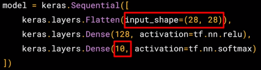
Remember last time we had a sequential with just one layer in it. Now we have three layers. The important things to look at are the first and the last layers. The last layer has 10 neurons in it because we have ten classes of clothing in the dataset. They should always match.
The first layer is a flatten layer with the input shaping 28 by 28. Now, if you remember our images are 28 by 28, so we're specifying that this is the shape that we should expect the data to be in. Flatten takes this 28 by 28 square and turns it into a simple linear array.

The interesting stuff happens in the middle layer, sometimes also called a hidden layer. This is 128 neurons in it, and I'd like you to think about these as variables in a function. Maybe call them x1, x2 x3, etc. Now, there exists a rule that incorporates all of these that turns the 784 values of an ankle boot into the value nine, and similar for all of the other 70,000. It's too complex a function for you to see by mapping the images yourself, but that's what a neural net does.
So, for example, if you then say the function was y equals w1 times x1, plus w2 times x2, plus w3 times x3, all the way up to a w128 times x128. By figuring out the values of w, then y will be nine when you have the input value of the shoe. You'll see that it's doing something very, very similar to what we did earlier when we figured out y equals 2x minus one. In that case, the two was the weight of x. So, I'm saying y equals w1 times x1, etc.
Now, don't worry if this isn't very clear right now. Over time, you will get the hang of it, seeing that it works, and there are also some tools that will allow you to peek inside to see what's going on. The important thing, for now, is to get the code working, so you can see a classification scenario for yourself. You can also tune the neural network by adding, removing and changing layer size to see the impact. You'll do that in the next exercise.

Also, if you want to go further, check out this tutorial from Andrew on YouTube, which will clarify how dense connected layer's work from the theoretical and mathematical perspective. But for now, let's get back to the code.
Walk through a Notebook for computer vision
Okay. So you just saw how to create a neural network that gives basic computer vision capabilities to recognize different items of clothing. Let's now work through a workbook that has all of the code to do that. You'll then go through this workbook yourself and if you want you can try some exercises.
Let's start by importing TensorFlow. I'm going to get the fashion MNIST data using tf.kares.datasets. By calling the load data method, I get training data and labels as well as test data and labels. For more details on these, check back to the previous video. The data for a particular image is a grid of values from zero to 255 with pixel Grayscale values. Using matplotlib, I can plot these as an image to make it easier to inspect. I can also print out the raw values so we can see what they look like. Here you can see the raw values for the pixel numbers from zero to 255, and here you can see the actual image. That was for the first image in the array. Let's take a look at the image at index 42 instead, and we can see the different pixel values and the actual graphic. Our image has values from zero to 255, but neural networks work better with normalized data.
So, let's change it to between zero and one simply by dividing every value by 255. In Python, you can actually divide an entire array with one line of code like this.
So now we design our model. As explained earlier, there's an input layer in the shape of the data and an output layer in the shape of the classes, and one hidden layer that tries to figure out the roles between them.
Now we compile the model to finding the loss function and the optimizer, and the goal of these is as before, to make a guess as to what the relationship is between the input data and the output data, measure how well or how badly it did using the loss function, use the optimizer to generate a new gas and repeat. We can then try to fit the training images to the training labels. We'll just do it for five epochs to be quick.
We spend about 25 seconds training it over five epochs and we end up with a loss of about 0.29. That means it's pretty accurate in guessing the relationship between the images and their labels. That's not great, but considering it was done in just 25 seconds with a very basic neural network, it's not bad either.
But a better measure of performance can be seen by trying the test data. These are images that the network has not yet seen. You would expect performance to be worse, but if it's much worse, you have a problem. As you can see, it's about 0.345 loss, meaning it's a little bit less accurate on the test set. It's not great either, but we know we're doing something right.
Your job now is to go through the workbook, try the exercises and see by tweaking the parameters on the neural network or changing the epochs, if there's a way for you to get it above 0.71 loss accuracy on training data and 0.66 accuracy on test data, give it a try for yourself.
Code: Fashion MNIST
Beyond Hello World, A Computer Vision Example
In the previous exercise, you saw how to create a neural network that figured out the problem you were trying to solve. This gave an explicit example of learned behavior. Of course, in that instance, it was a bit of overkill because it would have been easier to write the function Y=2x-1 directly, instead of bothering with using Machine Learning to learn the relationship between X and Y for a fixed set of values and extending that for all values.
But what about a scenario where writing rules like that is much more difficult -- for example a computer vision problem? Let's take a look at a scenario where we can recognize different items of clothing, trained from a dataset containing 10 different types.
Start Coding
Let's start with our import of TensorFlow
import tensorflow as tf
print(tf.__version__)
1.13.1
The Fashion MNIST data is available directly in the tf.keras datasets API. You load it like this:
mnist = tf.keras.datasets.fashion_mnistCalling load_data on this object will give you two sets of two lists, these will be the training and testing values for the graphics that contain the clothing items and their labels.
(training_images, training_labels), (test_images, test_labels) = mnist.load_data()Downloading data from https://storage.googleapis.com/tensorflow/tf-keras-datasets/train-labels-idx1-ubyte.gz
32768/29515 [=================================] - 0s 0us/step
40960/29515 [=========================================] - 0s 0us/step Downloading data from https://storage.googleapis.com/tensorflow/tf-keras-datasets/train-images-idx3-ubyte.gz
26427392/26421880 [==============================] - 0s 0us/step
26435584/26421880 [==============================] - 0s 0us/step Downloading data from https://storage.googleapis.com/tensorflow/tf-keras-datasets/t10k-labels-idx1-ubyte.gz
16384/5148 [===============================================================================================] - 0s 0us/step Downloading data from https://storage.googleapis.com/tensorflow/tf-keras-datasets/t10k-images-idx3-ubyte.gz 4423680/4422102 [==============================] - 0s 0us/step
4431872/4422102 [==============================] - 0s 0us/step
What does these values look like? Let's print a training image, and a training label to see...Experiment with different indices in the array. For example, also take a look at index 42...that's a a different boot than the one at index 0
import matplotlib.pyplot as plt
plt.imshow(training_images[0])
print(training_labels[0])
print(training_images[0])

You'll notice that all of the values in the number are between 0 and 255. If we are training a neural network, for various reasons it's easier if we treat all values as between 0 and 1, a process called '**normalizing**'...and fortunately in Python it's easy to normalize a list like this without looping. You do it like this:
training_images  = training_images / 255.0
test_images = test_images / 255.0
Now you might be wondering why there are 2 sets...training and testing -- remember we spoke about this in the intro? The idea is to have 1 set of data for training, and then another set of data...that the model hasn't yet seen...to see how good it would be at classifying values. After all, when you're done, you're going to want to try it out with data that it hadn't previously seen!
Let's now design the model. There's quite a few new concepts here, but don't worry, you'll get the hang of them.
model = tf.keras.models.Sequential([tf.keras.layers.Flatten(),
                                    tf.keras.layers.Dense(128, activation=tf.nn.relu),
tf.keras.layers.Dense(10, activation=tf.nn.softmax)])Sequential: That defines a SEQUENCE of layers in the neural network
Flatten: Remember earlier where our images were a square, when you printed them out? Flatten just takes that square and turns it into a 1 dimensional set.
Dense: Adds a layer of neurons
Each layer of neurons need an activation function to tell them what to do. There's lots of options, but just use these for now.
Relu effectively means "If X>0 return X, else return 0" -- so what it does it it only passes values 0 or greater to the next layer in the network.
Softmax takes a set of values, and effectively picks the biggest one, so, for example, if the output of the last layer looks like [0.1, 0.1, 0.05, 0.1, 9.5, 0.1, 0.05, 0.05, 0.05], it saves you from fishing through it looking for the biggest value, and turns it into [0,0,0,0,1,0,0,0,0] -- The goal is to save a lot of coding!
The next thing to do, now the model is defined, is to actually build it. You do this by compiling it with an optimizer and loss function as before -- and then you train it by calling model.fit asking it to fit your training data to your training labels -- i.e. have it figure out the relationship between the training data and its actual labels, so in future if you have data that looks like the training data, then it can make a prediction for what that data would look like.
model.compile(optimizer = tf.train.AdamOptimizer(),
              loss = 'sparse_categorical_crossentropy',
              metrics=['accuracy'])

model.fit(training_images, training_labels, epochs=5)
WARNING:tensorflow:From /usr/local/lib/python2.7/dist-packages/tensorflow/python/ops/resource_variable_ops.py:435: colocate_with (from tensorflow.python.framework.ops) is deprecated and will be removed in a future version. Instructions for updating: Colocations handled automatically by placer. Epoch 1/5 60000/60000 [==============================] - 6s 98us/sample - loss: 0.4959 - acc: 0.8240 Epoch 2/5 60000/60000 [==============================] - 5s 85us/sample - loss: 0.3747 - acc: 0.8644 Epoch 3/5 60000/60000 [==============================] - 5s 85us/sample - loss: 0.3377 - acc: 0.8759 Epoch 4/5 60000/60000 [==============================] - 5s 83us/sample - loss: 0.3131 - acc: 0.8854 Epoch 5/5 60000/60000 [==============================] - 5s 82us/sample - loss: 0.2925 - acc: 0.8914<tensorflow.python.keras.callbacks.History at 0x7f3df5b78910>
Once it's done training -- you should see an accuracy value at the end of the final epoch. It might look something like 0.9098. This tells you that your neural network is about 91% accurate in classifying the training data. I.E., it figured out a pattern match between the image and the labels that worked 91% of the time. Not great, but not bad considering it was only trained for 5 epochs and done quite quickly.
But how would it work with unseen data? That's why we have the test images. We can call model.evaluate, and pass in the two sets, and it will report back the loss for each. Let's give it a try:
model.evaluate(test_images, test_labels)10000/10000 [==============================] - 0s 48us/sample - loss: 0.3547 - acc: 0.8719[0.3547124492526054, 0.8719]
Exploration Exercises
Exercise 1:
For this first exercise run the below code: It creates a set of classifications for each of the test images, and then prints the first entry in the classifications. The output, after you run it is a list of numbers. Why do you think this is, and what do those numbers represent?
classifications = model.predict(test_images)

print(classifications[0])
[9.1596513e-07 9.6772510e-09 1.7723127e-07 3.3424172e-07 3.3442102e-08
2.8960702e-03 6.0414425e-07 1.7956610e-01 6.2276158e-05 8.1747347e-01]
Hint: try running print(test_labels[0]) -- and you'll get a 9. Does that help you understand why this list looks the way it does?
print(test_labels[0])9
What does this list represent?
- It's 10 random meaningless values
- It's the first 10 classifications that the computer made
- It's the probability that this item is each of the 10 classes
Answer:
The correct answer is (3)
The output of the model is a list of 10 numbers. These numbers are a probability that the value being classified is the corresponding value, i.e. the first value in the list is the probability that the handwriting is of a '0', the next is a '1' etc. Notice that they are all VERY LOW probabilities.
For the 7, the probability was .999+, i.e. the neural network is telling us that it's almost certainly a 7.
How do you know that this list tells you that the item is an ankle boot?
- There's not enough information to answer that question
- The 10th element on the list is the biggest, and the ankle boot is labelled 9
- The ankle boot is label 9, and there are 0->9 elements in the list
Answer
The correct answer is (2). Both the list and the labels are 0 based, so the ankle boot having label 9 means that it is the 10th of the 10 classes. The list having the 10th element being the highest value means that the Neural Network has predicted that the item it is classifying is most likely an ankle boot
Exercise 2:
Let's now look at the layers in your model. Experiment with different values for the dense layer with 512 neurons. What different results do you get for loss, training time etc? Why do you think that's the case?
import tensorflow as tf
print(tf.__version__)

mnist = tf.keras.datasets.mnist

(training_images, training_labels) ,  (test_images, test_labels) = mnist.load_data()

training_images = training_images/255.0
test_images = test_images/255.0

model = tf.keras.models.Sequential([tf.keras.layers.Flatten(),
                                    tf.keras.layers.Dense(1024, activation=tf.nn.relu),
                                    tf.keras.layers.Dense(10, activation=tf.nn.softmax)])

model.compile(optimizer = 'adam',
              loss = 'sparse_categorical_crossentropy')

model.fit(training_images, training_labels, epochs=5)

model.evaluate(test_images, test_labels)

classifications = model.predict(test_images)

print(classifications[0])
print(test_labels[0])
1.13.1 Downloading data from https://storage.googleapis.com/tensorflow/tf-keras-datasets/mnist.npz
11493376/11490434 [==============================] - 0s 0us/step 1
1501568/11490434 [==============================] - 0s 0us/step
Epoch 1/5 60000/60000 [==============================] - 28s 467us/sample - loss: 0.1850
Epoch 2/5 60000/60000 [==============================] - 27s 450us/sample - loss: 0.0738
Epoch 3/5 60000/60000 [==============================] - 28s 461us/sample - loss: 0.0479
Epoch 4/5 60000/60000 [==============================] - 27s 445us/sample - loss: 0.0354
Epoch 5/5 60000/60000 [==============================] - 28s 460us/sample - loss: 0.0261
10000/10000 [==============================] - 1s 100us/sample - loss: 0.0860
[8.3409720e-12 1.0426395e-09 5.7396080e-12 1.4494176e-06 1.8278910e-16
6.5416081e-13 5.3156525e-17 9.9999857e-01 1.0763074e-12 3.9761030e-09]
7
Question 1. Increase to 1024 Neurons -- What's the impact?
- Training takes longer but is more accurate
- Training takes longer, but no impact on accuracy
- Training takes the same time but is more accurate
Answer
The correct answer is (1) by adding more Neurons we have to do more calculations, slowing down the process, but in this case they have a good impact -- we do get more accurate. That doesn't mean it's always a case of 'more is better', you can hit the law of diminishing returns very quickly!
Exercise 3:
What would happen if you remove the Flatten() layer? Why do you think that's the case?
You get an error about the shape of the data. It may seem vague right now, but it reinforces the rule of thumb that the first layer in your network should be the same shape as your data. Right now our data is 28x28 images, and 28 layers of 28 neurons would be infeasible, so it makes more sense to 'flatten' that 28,28 into a 784x1. Instead of wriitng all the code to handle that ourselves, we add the Flatten() layer at the begining, and when the arrays are loaded into the model later, they'll automatically be flattened for us.
import tensorflow as tf
print(tf.__version__)

mnist = tf.keras.datasets.mnist

(training_images, training_labels) ,  (test_images, test_labels) = mnist.load_data()

training_images = training_images/255.0
test_images = test_images/255.0

model = tf.keras.models.Sequential([#tf.keras.layers.Flatten(),
                                    tf.keras.layers.Dense(64, activation=tf.nn.relu),
                                    tf.keras.layers.Dense(10, activation=tf.nn.softmax)])

model.compile(optimizer = 'adam',
              loss = 'sparse_categorical_crossentropy')

model.fit(training_images, training_labels, epochs=5)

model.evaluate(test_images, test_labels)

classifications = model.predict(test_images)

print(classifications[0])
print(test_labels[0])
InvalidArgumentError: logits and labels must have the same first dimension, got logits shape [896,10] and labels shape [32] [[{{node loss_3/output_1_loss/SparseSoftmaxCrossEntropyWithLogits/SparseSoftmaxCrossEntropyWithLogits}}]]
Exercise 4:
Consider the final (output) layers. Why are there 10 of them? What would happen if you had a different amount than 10? For example, try training the network with 5
You get an error as soon as it finds an unexpected value. Another rule of thumb -- the number of neurons in the last layer should match the number of classes you are classifying for. In this case, it's the digits 0-9, so there are 10 of them, hence you should have 10 neurons in your final layer.
import tensorflow as tf
print(tf.__version__)

mnist = tf.keras.datasets.mnist

(training_images, training_labels) ,  (test_images, test_labels) = mnist.load_data()

training_images = training_images/255.0
test_images = test_images/255.0

model = tf.keras.models.Sequential([tf.keras.layers.Flatten(),
                                    tf.keras.layers.Dense(64, activation=tf.nn.relu),
                                    tf.keras.layers.Dense(5, activation=tf.nn.softmax)])

model.compile(optimizer = 'adam',
              loss = 'sparse_categorical_crossentropy')

model.fit(training_images, training_labels, epochs=5)

model.evaluate(test_images, test_labels)

classifications = model.predict(test_images)

print(classifications[0])
print(test_labels[0])
InvalidArgumentError: Received a label value of 9 which is outside the valid range of [0, 5). Label values: 8 4 3 5 9 8 5 1 7 7 8 7 6 3 4 9 7 3 8 2 1 3 1 1 8 3 6 3 8 5 3 8 [[{{node loss_4/output_1_loss/SparseSoftmaxCrossEntropyWithLogits/SparseSoftmaxCrossEntropyWithLogits}}]]
Exercise 5:
Consider the effects of additional layers in the network. What will happen if you add another layer between the one with 512 and the final layer with 10.
Ans: There isn't a significant impact -- because this is relatively simple data. For far more complex data (including color images to be classified as flowers that you'll see in the next lesson), extra layers are often necessary.
import tensorflow as tf
print(tf.__version__)

mnist = tf.keras.datasets.mnist

(training_images, training_labels) ,  (test_images, test_labels) = mnist.load_data()

training_images = training_images/255.0
test_images = test_images/255.0

model = tf.keras.models.Sequential([tf.keras.layers.Flatten(),
                                    tf.keras.layers.Dense(512, activation=tf.nn.relu),
                                    tf.keras.layers.Dense(256, activation=tf.nn.relu),
                                    tf.keras.layers.Dense(5, activation=tf.nn.softmax)])

model.compile(optimizer = 'adam',
              loss = 'sparse_categorical_crossentropy')

model.fit(training_images, training_labels, epochs=5)

model.evaluate(test_images, test_labels)

classifications = model.predict(test_images)

print(classifications[0])
print(test_labels[0])
InvalidArgumentError: Received a label value of 9 which is outside the valid range of [0, 5). Label values: 4 0 3 3 2 5 9 5 2 2 3 1 2 5 8 3 6 5 0 1 3 1 3 7 1 1 0 8 7 6 3 0 [[{{node loss_5/output_1_loss/SparseSoftmaxCrossEntropyWithLogits/SparseSoftmaxCrossEntropyWithLogits}}]]
Exercise 6:
Consider the impact of training for more or less epochs. Why do you think that would be the case?
Try 15 epochs -- you'll probably get a model with a much better loss than the one with 5 Try 30 epochs -- you might see the loss value stops decreasing, and sometimes increases. This is a side effect of something called 'overfitting' which you can learn about [somewhere] and it's something you need to keep an eye out for when training neural networks. There's no point in wasting your time training if you aren't improving your loss, right! :)
import tensorflow as tf
print(tf.__version__)

mnist = tf.keras.datasets.mnist

(training_images, training_labels) ,  (test_images, test_labels) = mnist.load_data()

training_images = training_images/255.0
test_images = test_images/255.0

model = tf.keras.models.Sequential([tf.keras.layers.Flatten(),
                                    tf.keras.layers.Dense(128, activation=tf.nn.relu),
                                    tf.keras.layers.Dense(5, activation=tf.nn.softmax)])

model.compile(optimizer = 'adam',
              loss = 'sparse_categorical_crossentropy')

model.fit(training_images, training_labels, epochs=30)

model.evaluate(test_images, test_labels)

classifications = model.predict(test_images)

print(classifications[34])
print(test_labels[34])
InvalidArgumentError: Received a label value of 9 which is outside the valid range of [0, 5). Label values: 4 2 3 4 2 8 3 4 1 2 9 3 9 9 8 2 1 4 6 6 7 4 5 2 9 1 4 5 2 6 2 3 [[{{node loss_6/output_1_loss/SparseSoftmaxCrossEntropyWithLogits/SparseSoftmaxCrossEntropyWithLogits}}]]
Exercise 7:
Before you trained, you normalized the data, going from values that were 0-255 to values that were 0-1. What would be the impact of removing that? Here's the complete code to give it a try. Why do you think you get different results?
import tensorflow as tf
print(tf.__version__)
mnist = tf.keras.datasets.mnist
(training_images, training_labels), (test_images, test_labels) = mnist.load_data()
training_images=training_images/255.0
test_images=test_images/255.0
model = tf.keras.models.Sequential([
  tf.keras.layers.Flatten(),
  tf.keras.layers.Dense(512, activation=tf.nn.relu),
  tf.keras.layers.Dense(10, activation=tf.nn.softmax)
])
model.compile(optimizer='adam', loss='sparse_categorical_crossentropy')
model.fit(training_images, training_labels, epochs=5)
model.evaluate(test_images, test_labels)
classifications = model.predict(test_images)
print(classifications[0])
print(test_labels[0])
1.13.1
Epoch 1/5 60000/60000 [==============================] - 19s 311us/sample - loss: 0.2008
Epoch 2/5 60000/60000 [==============================] - 18s 308us/sample - loss: 0.0820
Epoch 3/5 60000/60000 [==============================] - 18s 296us/sample - loss: 0.0530
Epoch 4/5 60000/60000 [==============================] - 18s 295us/sample - loss: 0.0367
Epoch 5/5 60000/60000 [==============================] - 18s 294us/sample - loss: 0.0290
10000/10000 [==============================] - 1s 91us/sample - loss: 0.0680
[3.9249587e-10 2.1030559e-10 6.9143766e-08 1.1339203e-07 9.4936584e-14
8.9032559e-10 1.6588608e-13 9.9999976e-01 3.5548162e-10 2.8273357e-08]
7
Exercise 8:
Earlier when you trained for extra epochs you had an issue where your loss might change. It might have taken a bit of time for you to wait for the training to do that, and you might have thought 'wouldn't it be nice if I could stop the training when I reach a desired value?' -- i.e. 95% accuracy might be enough for you, and if you reach that after 3 epochs, why sit around waiting for it to finish a lot more epochs....So how would you fix that? Like any other program...you have callbacks! Let's see them in action...
import tensorflow as tf
print(tf.__version__)

class myCallback(tf.keras.callbacks.Callback):
  def on_epoch_end(self, epoch, logs={}):
    if(logs.get('loss')<0.4):
      print("\nReached 60% accuracy so cancelling training!")
      self.model.stop_training = True

callbacks = myCallback()
mnist = tf.keras.datasets.fashion_mnist
(training_images, training_labels), (test_images, test_labels) = mnist.load_data()
training_images=training_images/255.0
test_images=test_images/255.0
model = tf.keras.models.Sequential([
  tf.keras.layers.Flatten(),
  tf.keras.layers.Dense(512, activation=tf.nn.relu),
  tf.keras.layers.Dense(10, activation=tf.nn.softmax)
])
model.compile(optimizer='adam', loss='sparse_categorical_crossentropy')
model.fit(training_images, training_labels, epochs=5, callbacks=[callbacks])
1.13.1
Epoch 1/5
60000/60000 [==============================] - 17s 289us/sample - loss: 0.4761
Epoch 2/5
59936/60000 [============================>.] - ETA: 0s - loss: 0.3574
Reached 60% accuracy so cancelling training!
60000/60000 [==============================] - 16s 274us/sample - loss: 0.3573
<tensorflow.python.keras.callbacks.History at 0x7f3dc3260210>
Using Callbacks to control training
A question I often get at this point from programmers in particular when experimenting with different numbers of epochs is, How can I stop training when I reach a point that I want to be at? What do I always have to hard code it to go for certain number of epochs? Well, the good news is that, the training loop does support callbacks. So in every epoch, you can callback to a code function, having checked the metrics. If they're what you want to say, then you can cancel the training at that point.

Let's take a look. Okay, so here's our code for training the neural network to recognize the fashion images. In particular, keep an eye on the model.fit function that executes the training loop. You can see that here.

What we'll now do is write a callback in Python. Here's the code. It's implemented as a separate class, but that can be in-line with your other code. It doesn't need to be in a separate file. In it, we'll implement the on_epoch_end function, which gets called by the callback whenever the epoch ends. It also sends a logs object which contains lots of great information about the current state of training. For example, the current loss is available in the logs, so we can query it for a certain amount. For example, here I'm checking if the loss is less than 0.4 and canceling the training itself. Now that we have our callback, let's return to the rest of the code, and there are two modifications that we need to make.

First, we instantiate the class that we just created, we do that with this code. Then, in my model.fit, I used the callbacks parameter and pass it this instance of the class. Let's see this in action.
import tensorflow as tf

class myCallback(tf.keras.callbacks.Callback):
  def on_epoch_end(self, epoch, logs={}):
    if(logs.get('acc')>0.6):
      print("\nReached 60% accuracy so cancelling training!")
      self.model.stop_training = True

mnist = tf.keras.datasets.fashion_mnist

(x_train, y_train),(x_test, y_test) = mnist.load_data()
x_train, x_test = x_train / 255.0, x_test / 255.0

callbacks = myCallback()

model = tf.keras.models.Sequential([
  tf.keras.layers.Flatten(input_shape=(28, 28)),
  tf.keras.layers.Dense(512, activation=tf.nn.relu),
  tf.keras.layers.Dense(10, activation=tf.nn.softmax)
])
model.compile(optimizer='adam',
              loss='sparse_categorical_crossentropy',
              metrics=['accuracy'])

model.fit(x_train, y_train, epochs=10, callbacks=[callbacks])
Walk through a notebook with Callbacks
Let's take a look at the code for callbacks, and see how it works. You can see the code here. Here's the notebook with the code already written, and here's the class that we defined to handle the callback, and here is where we instantiate the callback class itself. Finally, here's where we set up the callback to be called as part of the training loop. As we begin training, note that we asked it to train for five epochs. Now, keep an eye on the losses that trains. We want to break when it goes below 0.4, and by the end of the first epoch we're actually getting close already. As the second epoch begins, it has already dropped below 0.4, but the callback hasn't been hit yet. That's because we set it up for on epoch end. It's good practice to do this, because with some data and some algorithms, the loss may vary up and down during the epoch, because all of the data hasn't yet been processed. So, I like to wait for the end to be sure. Now the epoch has ended, and the loss is 0.3563, and we can see that the training ends, even though we've only done two epochs. Note that we're sure we asked for five epochs and that we ended after two, because the loss is below 0.4, which we checked for in the callback. It's pretty cool right?
Downloading data from https://storage.googleapis.com/tensorflow/tf-keras-datasets/train-labels-idx1-ubyte.gz
32768/29515 [=================================] - 0s 0us/step
Downloading data from https://storage.googleapis.com/tensorflow/tf-keras-datasets/train-images-idx3-ubyte.gz
26427392/26421880 [==============================] - 0s 0us/step
Downloading data from https://storage.googleapis.com/tensorflow/tf-keras-datasets/t10k-labels-idx1-ubyte.gz
8192/5148 [===============================================] - 0s 0us/step
Downloading data from https://storage.googleapis.com/tensorflow/tf-keras-datasets/t10k-images-idx3-ubyte.gz
4423680/4422102 [==============================] - 0s 0us/step
WARNING:tensorflow:From /usr/local/lib/python3.6/dist-packages/tensorflow/python/ops/resource_variable_ops.py:435: colocate_with (from tensorflow.python.framework.ops) is deprecated and will be removed in a future version.
Instructions for updating:
Colocations handled automatically by placer.
Epoch 1/10
59808/60000 [============================>.] - ETA: 0s - loss: 0.4722 - acc: 0.8316
Reached 60% accuracy so cancelling training!
60000/60000 [==============================] - 17s 278us/sample - loss: 0.4721 - acc: 0.8315
<tensorflow.python.keras.callbacks.History at 0x7f14b01eabe0>
Week 2 Quiz


![]()
codes: