【ML】之 线性回归（实战） 研读

 原文：https://blog.csdn.net/fanfan4569/article/details/81263499

Topic:

1. 最小二乘法代数求解 实战
2. 最小二乘法矩阵求解 实战
3. 使用 scikit-learn 进行线性回归预测

本文为实战篇，理论篇：线性回归理论

 一、最小二乘法代数求解 实战

步骤：

1. 导入数据集（使用 numpy模拟）
2. 绘制图形， 使用matplotlib
3. 定义拟合直线函数，平方损失函数
4. 计算求解
5. 绘制图像
6. 测试用例，预测结果

# 1. 导入数据集
#import inline as inline
import matplotlib
import numpy as np

x = np.array([56, 72, 69, 88, 102, 86, 76, 79, 94, 74])
y = np.array([92, 102, 86, 110, 130, 99, 96, 102, 105, 92])

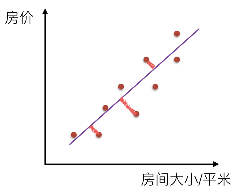
# 2. 显示数据集在坐标上
from matplotlib import pyplot as plt
# %matplotlib inline

plt.scatter(x, y)
plt.xlabel("Area")
plt.ylabel("Price")
plt.show()


# 3. 定义拟合直线
def f(x, b, w1):
    y = b + w1 * x
    return y

# 3.2 平方损失函数
def square_loss(x, y, w0, w1):
    loss = sum(np.square(y - (w0 + w1*x)))
    return loss

# 3.4 代入计算

b,w = w_calculator(x, y)

square_loss(x, y, b, w)

# 4. 绘制图像 
x_temp = np.linspace(50,120,100) # 绘制直线生成的临时点 
plt.scatter(x, y) 
plt.plot(x_temp, x_temp*w + b, 'r') 
plt.show() # 5. 如果手中有一套 150 平米的房产想售卖，

二、最小二乘法矩阵求解 实战

步骤：

1. 导入数据集
2. 定义 拟合直线，平方损失函数
3. 代入计算
4. 绘图

# 1. 导入数据集
import inline as inline
import matplotlib
import numpy as np

x = np.array([56, 72, 69, 88, 102, 86, 76, 79, 94, 74])
y = np.array([92, 102, 86, 110, 130, 99, 96, 102, 105, 92])

# 2. 显示数据集在坐标上
from matplotlib import pyplot as plt
# %matplotlib inline

plt.scatter(x, y)
plt.xlabel("Area")
plt.ylabel("Price")
plt.show()


# 3. 定义拟合直线
def f(x, b, w1):
    y = b + w1 * x
    return y

# 3.2 平方损失函数
def square_loss(x, y, w0, w1):
    loss = sum(np.square(y - (w0 + w1*x)))
    return loss

# 3.3 平方损失函数最小时对应的w参数值 ，b 

def w_calculator(x, y): 
n = len(x) 
w1 = (n*sum(x*y) - sum(x)*sum(y))/(n*sum(x*x) - sum(x)*sum(x)) 
w0 = (sum(x*x)*sum(y) - sum(x)*sum(x*y))/(n*sum(x*x)-sum(x)*sum(x)) 
return w0, w1


# 3.4 代入计算

b,w w_calculator(x, y)
square_loss(x, y, b, w)

# 4. 绘制图像
x_temp = np.linspace(50,120,100) # 绘制直线生成的临时点
plt.scatter(x, y)
plt.plot(x_temp, x_temp*w + b, 'r')
plt.show()


# 5. 如果手中有一套 150 平米的房产想售卖，获取预估报价：
f(150, b, w)

三、使用 scikit-learn 进行线性回归预测

scikit-learn 实现最小二乘线性回归方法 

这要用到

LinearRegression(),sklearn.linear_model.LinearRegression(fit_intercept=True, normalize=False, copy_X=True, n_jobs=1)

fit_intercept: 默认为 True，计算截距项。
normalize: 默认为 False，不针对数据进行标准化处理。
copy_X: 默认为 True，即使用数据的副本进行操作，防止影响原数据。
n_jobs: 计算时的作业数量。默认为 1，若为 -1 则使用全部 CPU 参与运算。
 

from sklearn.linear_model import LinearRegression
import numpy as np
import scipy # 要导入scipy包，不然报错

# 1. 定义数据集
x = np.array([56, 72, 69, 88, 102, 86, 76, 79, 94, 74])
y = np.array([92, 102, 86, 110, 130, 99, 96, 102, 105, 92])


# 2. 定义线性回归模型
model = LinearRegression()
# 训练, reshape 操作把数据处理成 fit 能接受的形状
model.fit(x.reshape(len(x), 1), y)

# 3.得到模型拟合参数
model.intercept_, model.coef_

# 4. 预测
model.predict([[150]])

实战1：https://blog.csdn.net/txbsw/article/details/79046362

实战2：https://blog.csdn.net/kyriehe/article/details/77507473

一元线性回归：

 

多元线性回归：