学习spark ml源码——线性回归

1、参数配置相关代码

/**
 * Params for linear regression.
 */
private[regression] trait LinearRegressionParams extends PredictorParams
    with HasRegParam with HasElasticNetParam with HasMaxIter with HasTol
    with HasFitIntercept with HasStandardization with HasWeightCol with HasSolver
    with HasAggregationDepth {

  import LinearRegression._

  /**
   * The solver algorithm for optimization.
   * Supported options: "l-bfgs", "normal" and "auto".
   * Default: "auto"
   *
   * @group param
   */
  @Since("1.6.0")
  final override val solver: Param[String] = new Param[String](this, "solver",
    "The solver algorithm for optimization. Supported options: " +
      s"${supportedSolvers.mkString(", ")}. (Default auto)",
    ParamValidators.inArray[String](supportedSolvers))
}

LinearRegressionParams 该类继承了PredictorParams中的各个特征trait，“private[regression]”表明该类是私有的，只能在regression包中才可以访问。这里有关trait相关的内容可以访问scala入门教程：scala中的trait进行学习，这里先不详细解释，后续有时间专门开一个博客进行总结学习。“final override val solver”的final与val表明solver是一个不能被重写的常量，override表明该常量在这里被重写。
这里scala语法有三点需要注意：
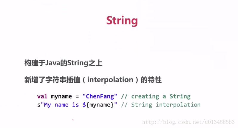
1）scala的string类型

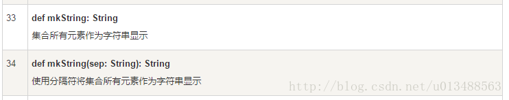
2）Scala Set 常用方法

3）SCALA中this关键字。这里暂时没怎么明白，希望在以后的学习中能够理解。
接下来就是各种参数的配置说明，这里不做详细解释，仔细看英文都可以明白。

/**
 * Linear regression.
 *
 * The learning objective is to minimize the squared error, with regularization.
 * The specific squared error loss function used is:
 *
 * <blockquote>
 *    $$
 *    L = 1/2n ||A coefficients - y||^2^
 *    $$
 * </blockquote>
 *
 * This supports multiple types of regularization:
 *  - none (a.k.a. ordinary least squares)
 *  - L2 (ridge regression)
 *  - L1 (Lasso)
 *  - L2 + L1 (elastic net)
 */
@Since("1.3.0")
class LinearRegression @Since("1.3.0") (@Since("1.3.0") override val uid: String)
  extends Regressor[Vector, LinearRegression, LinearRegressionModel]
  with LinearRegressionParams with DefaultParamsWritable with Logging {

  import LinearRegression._

  @Since("1.4.0")
  def this() = this(Identifiable.randomUID("linReg"))

  /**
   * Set the regularization parameter.
   * Default is 0.0.
   *
   * @group setParam
   */
  @Since("1.3.0")
  def setRegParam(value: Double): this.type = set(regParam, value)
  setDefault(regParam -> 0.0)

  /**
   * Set if we should fit the intercept.
   * Default is true.
   *
   * @group setParam
   */
  @Since("1.5.0")
  def setFitIntercept(value: Boolean): this.type = set(fitIntercept, value)
  setDefault(fitIntercept -> true)

  /**
   * Whether to standardize the training features before fitting the model.
   * The coefficients of models will be always returned on the original scale,
   * so it will be transparent for users.
   * Default is true.
   *
   * @note With/without standardization, the models should be always converged
   * to the same solution when no regularization is applied. In R's GLMNET package,
   * the default behavior is true as well.
   *
   * @group setParam
   */
  @Since("1.5.0")
  def setStandardization(value: Boolean): this.type = set(standardization, value)
  setDefault(standardization -> true)

  /**
   * Set the ElasticNet mixing parameter.
   * For alpha = 0, the penalty is an L2 penalty.
   * For alpha = 1, it is an L1 penalty.
   * For alpha in (0,1), the penalty is a combination of L1 and L2.
   * Default is 0.0 which is an L2 penalty.
   *
   * @group setParam
   */
  @Since("1.4.0")
  def setElasticNetParam(value: Double): this.type = set(elasticNetParam, value)
  setDefault(elasticNetParam -> 0.0)

  /**
   * Set the maximum number of iterations.
   * Default is 100.
   *
   * @group setParam
   */
  @Since("1.3.0")
  def setMaxIter(value: Int): this.type = set(maxIter, value)
  setDefault(maxIter -> 100)

  /**
   * Set the convergence tolerance of iterations.
   * Smaller value will lead to higher accuracy with the cost of more iterations.
   * Default is 1E-6.
   *
   * @group setParam
   */
  @Since("1.4.0")
  def setTol(value: Double): this.type = set(tol, value)
  setDefault(tol -> 1E-6)

  /**
   * Whether to over-/under-sample training instances according to the given weights in weightCol.
   * If not set or empty, all instances are treated equally (weight 1.0).
   * Default is not set, so all instances have weight one.
   *
   * @group setParam
   */
  @Since("1.6.0")
  def setWeightCol(value: String): this.type = set(weightCol, value)

  /**
   * Set the solver algorithm used for optimization.
   * In case of linear regression, this can be "l-bfgs", "normal" and "auto".
   *  - "l-bfgs" denotes Limited-memory BFGS which is a limited-memory quasi-Newton
   *    optimization method.
   *  - "normal" denotes using Normal Equation as an analytical solution to the linear regression
   *    problem.  This solver is limited to `LinearRegression.MAX_FEATURES_FOR_NORMAL_SOLVER`.
   *  - "auto" (default) means that the solver algorithm is selected automatically.
   *    The Normal Equations solver will be used when possible, but this will automatically fall
   *    back to iterative optimization methods when needed.
   *
   * @group setParam
   */
  @Since("1.6.0")
  def setSolver(value: String): this.type = set(solver, value)
  setDefault(solver -> Auto)

  /**
   * Suggested depth for treeAggregate (greater than or equal to 2).
   * If the dimensions of features or the number of partitions are large,
   * this param could be adjusted to a larger size.
   * Default is 2.
   *
   * @group expertSetParam
   */
  @Since("2.1.0")
  def setAggregationDepth(value: Int): this.type = set(aggregationDepth, value)
  setDefault(aggregationDepth -> 2)

2、训练模型相关代码

  override protected def train(dataset: Dataset[_]): LinearRegressionModel = {
    // Extract the number of features before deciding optimization solver.这里就是获取特征维度以及特征权重
    val numFeatures = dataset.select(col($(featuresCol))).first().getAs[Vector](0).size
    val w = if (!isDefined(weightCol) || $(weightCol).isEmpty) lit(1.0) else col($(weightCol))
//将模型需要的数据dataset转换为rdd的数据结构
    val instances: RDD[Instance] = dataset.select(
      col($(labelCol)), w, col($(featuresCol))).rdd.map {
      case Row(label: Double, weight: Double, features: Vector) =>
        Instance(label, weight, features)
    }
//获取各个参数配置信息
    val instr = Instrumentation.create(this, dataset)
    instr.logParams(labelCol, featuresCol, weightCol, predictionCol, solver, tol,
      elasticNetParam, fitIntercept, maxIter, regParam, standardization, aggregationDepth)
    instr.logNumFeatures(numFeatures)
//当样本的特征维度小于4096并且solver为auto或者solver为normal时，用WeightedLeastSquares求解，这是因为WeightedLeastSquares只需要处理一次数据， 求解效率更高。WeightedLeastSquares的介绍见[带权最小二乘](https://github.com/endymecy/spark-ml-source-analysis/blob/master/%E6%9C%80%E4%BC%98%E5%8C%96%E7%AE%97%E6%B3%95/WeightsLeastSquares.md)。
    if (($(solver) == Auto &&
      numFeatures <= WeightedLeastSquares.MAX_NUM_FEATURES) || $(solver) == Normal) {
      // For low dimensional data, WeightedLeastSquares is more efficient since the
      // training algorithm only requires one pass through the data. (SPARK-10668)

      val optimizer = new WeightedLeastSquares($(fitIntercept), $(regParam),
        elasticNetParam = $(elasticNetParam), $(standardization), true,
        solverType = WeightedLeastSquares.Auto, maxIter = $(maxIter), tol = $(tol))
      val model = optimizer.fit(instances)
      // When it is trained by WeightedLeastSquares, training summary does not
      // attach returned model.
      val lrModel = copyValues(new LinearRegressionModel(uid, model.coefficients, model.intercept))
      val (summaryModel, predictionColName) = lrModel.findSummaryModelAndPredictionCol()
      val trainingSummary = new LinearRegressionTrainingSummary(
        summaryModel.transform(dataset),
        predictionColName,
        $(labelCol),
        $(featuresCol),
        summaryModel,
        model.diagInvAtWA.toArray,//此参数的意义？？
        model.objectiveHistory)

      lrModel.setSummary(Some(trainingSummary))//Some函数？？
      instr.logSuccess(lrModel)
      return lrModel
    }

此段训练模型的代码总的来说是输入dataset，返回LinearRegressionModel 。
这里LeastSquaresAggregator用来计算最小二乘损失函数的梯度和损失。为了在优化过程中提高收敛速度，防止大方差 的特征在训练时产生过大的影响，将特征缩放到单元方差并且减去均值，可以减少条件数。当使用截距进行训练时，处在缩放后空间的目标函数 如下：

$$\begin{align} L &= 1/2N ||\sum_i w_i(x_i - \bar{x_i}) / \hat{x_i} - (y - \bar{y}) / \hat{y}||^2 \end{align}$$
  在这个公式中， $\bar{x_i}$是 $x_i$的均值， $\hat{x_i}$是 $x_i$的标准差， $\bar{y}$是标签的均值， $\hat{y}$ 是标签的标准差。

  如果不使用截距，我们可以使用同样的公式。不同的是$\bar{y}$和$\bar{x_i}$分别用0代替。这个公式可以重写为如下的形式。

$$\begin{align} L &= 1/2N ||\sum_i (w_i/\hat{x_i})x_i - \sum_i (w_i/\hat{x_i})\bar{x_i} - y / \hat{y} + \bar{y} / \hat{y}||^2 \\ &= 1/2N ||\sum_i w_i^\prime x_i - y / \hat{y} + offset||^2 = 1/2N diff^2 \end{align}$$
  在这个公式中， $w_i^\prime$是有效的相关系数，通过 $w_i/\hat{x_i}$计算。offset是 $- \sum_i (w_i/\hat{x_i})\bar{x_i} + \bar{y} / \hat{y}$， 而diff是 $\sum_i w_i^\prime x_i - y / \hat{y} + offset$。

  注意，相关系数和offset不依赖于训练数据集，所以它们可以提前计算。

  现在，目标函数的一阶导数如下所示：

$$\begin{align} \frac{\partial L}{\partial w_i} &= diff/N (x_i - \bar{x_i}) / \hat{x_i} \end{align}$$
  然而， $(x_i - \bar{x_i})$是一个密集的计算，当训练数据集是稀疏的格式时，这不是一个理想的公式。通过添加一个稠密项 $\bar{x_i} / \hat{x_i}$到 公式的末尾可以解决这个问题。目标函数的一阶导数如下所示：

$$\begin{align} \frac{\partial L}{\partial w_i} &=1/N \sum_j diff_j (x_{ij} - \bar{x_i}) / \hat{x_i} \\ &= 1/N ((\sum_j diff_j x_{ij} / \hat{x_i}) - diffSum \bar{x_i} / \hat{x_i}) \\ &= 1/N ((\sum_j diff_j x_{ij} / \hat{x_i}) + correction_i) \end{align}$$
  这里， $correction_i = - diffSum \bar{x_i} / \hat{x_i}$。通过一个简单的数学推导，我们就可以知道diffSum实际上为0。

$$\begin{align} diffSum &= \sum_j (\sum_i w_i(x_{ij} - \bar{x_i}) / \hat{x_i} - (y_j - \bar{y}) / \hat{y}) \\ &= N * (\sum_i w_i(\bar{x_i} - \bar{x_i}) / \hat{x_i} - (\bar{y} - \bar{y}) / \hat{y}) \\ &= 0 \end{align}$$
  所以，目标函数的一阶导数仅仅依赖于训练数据集，我们可以简单的通过分布式的方式来计算，并且对稀疏格式也很友好。

$$\begin{align} \frac{\partial L}{\partial w_i} &= 1/N ((\sum_j diff_j x_{ij} / \hat{x_i}) \end{align}$$
  我们首先看有效系数 $w_i/\hat{x_i}$和offset的实现。