正则化 regularization

点击此处返回总目录

有时候我们发现模型在训练数据集上的正确率非常高，但这个模型却很难对从未见过的数据做出正确相应。我们说，这个模型存在过拟合现象。

使用正则化方法可以有效缓解过拟合。也就是在损失函数中引入模型复杂度指标，给每个参数w加上权重，抑制训练数据中的噪声。

正则化通常只对参数w使用，不对偏置b使用。

使用正则化后，loss变成两部分。第一部分是以前求得的loss值，这一部分描述了正确结果与预测结果之间的差距，比如交叉熵、均方误差等。第二部分，用超参数REGULARIZER表示loss(w)的权重。

扫描二维码关注公众号，回复： 5506800 查看本文章

loss(w)有两种计算方式，一种是对所有w的绝对值求和，另一种是对所有w的平方的绝对追求和。这两种分别叫做L1正则化和L2正则化。TensorFlow中给出了两个函数，分别实现L1正则化实现和L2正则化实现。使用时，选择其中一个即可。

我们用tf.add_to_collection()把计算好的所有w正则化加在'losses'集合中。

用tf.add_n()可以把'losses'中的所有值相加。再加上交叉熵cem，构成了总损失函数。

我们感受一下正则化的作用。

生成一套数据集，随机产生300个符合正态分布的点[x0,x1]。把平方和<2的点标注为1，把其他点标注为0。

我们尝试拟合一条曲线，把蓝色的点和红色的点分开。

代码：

import tensorflow as tf
import numpy as np
import matplotlib.pyplot as plt

BATCH_SIZE = 30 #定义一次喂入的数据为30个
seed = 2

#################1.建立数据集，并画出可视化的散点#####################
#基于seed产生随机数
rng = np.random.RandomState(seed)
X = rng.randn(300,2) #300行2列。均值为0，方差为1的正态分布数据。
Y_=[int(x0*x0+x1*x1 < 2) for (x0,x1) in X] #若平方和<2，则标注为1，赋给Y_;否则标注为0，赋给Y_
Y_c =[['red' if y else 'blue']for y in Y_] #遍历Y_，如果不为0，标注为'red'；为0标注为'blue'

X = np.vstack(X).reshape(-1,2) #让X是n行两列。
Y_ = np.vstack(Y_).reshape(-1,1) #让Y_是n行一列。

print(X)
print(Y_)
print(Y_c)

plt.scatter(X[:,0],X[:,1],c=np.squeeze(Y_c)) #从Y_c中取对应颜色赋给c
plt.show()

##################2. 定义神经网络的输入输出参数，定义前向传播过程########
def get_weight(shape,regularizer): #为了方便，定义了一个生成参数w的函数。参数为shape和正则化权重。
w=tf.Variable(tf.random_normal(shape),dtype=tf.float32)
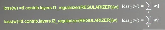
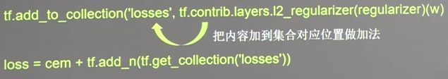
tf.add_to_collection('losses',tf.contrib.layers.l2_regularizer(regularizer)(w))
return w

def get_bias(shape):
b=tf.Variable(tf.constant(0.01,shape=shape))
return b

x=tf.placeholder(tf.float32,shape=(None,2))
y_=tf.placeholder(tf.float32,shape=(None,1))

w1=get_weight([2,11],0.01) #w1为2行11列。注意shape是列表的形式给出的。正则化权重为0.01
b1=get_bias([11])

y1=tf.nn.relu(tf.matmul(x,w1)+b1)

w2=get_weight([11,1],0.01)
b2=get_bias([1])

y=tf.matmul(y1,w2)+b2 #输出层不过激活函数

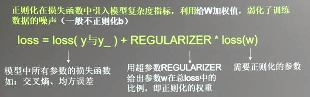
##################3. 定义损失函数#############
#定义损失函数
loss_mse = tf.reduce_mean(tf.square(y-y_)) #均方误差损失函数
loss_total = loss_mse + tf.add_n(tf.get_collection('losses')) #均方误差损失函数，加上每一个正则化w的损失

#################4.1 定义反向传播过程：不含正则化。########################
train_step = tf.train.AdamOptimizer(0.0001).minimize(loss_mse) #这个损失函数不包括正则化

with tf.Session() as sess:
init_op = tf.global_variables_initializer()
sess.run(init_op)
STEPS = 40000
for i in range(STEPS):
start = (i*BATCH_SIZE) % 300
end = start + BATCH_SIZE
sess.run(train_step,feed_dict={x:X[start:end],y_:Y_[start:end]})
if i%2000 ==0:
loss_mse_v = sess.run(loss_mse,feed_dict={x:X,y_:Y_}) #每2000轮打印一下loss值
print("After %d steps,loss is: %f" %(i,loss_mse_v))

xx,yy = np.mgrid[-3:3:0.01,-3:3:0.01] #生成网格坐标点
grid = np.c_[xx.ravel(),yy.ravel()] #将xx,yy拉直，合并成一个2列的矩阵，得到一个网格坐标点的集合
probs = sess.run(y,feed_dict={x:grid}) #将网格坐标点喂入神经网络，probs为输出
probs = probs.reshape(xx.shape) #probs的shape调整成xx的样子
print("w1:",sess.run(w1))
print("w2:",sess.run(b1))
print("w3:",sess.run(w2))
print("w4:",sess.run(b2))

plt.scatter(X[:,0],X[:,1],c=np.squeeze(Y_c))
plt.contour(xx,yy,probs,levels=[.5]) #给所有值为0.5的点上色
plt.show()

#####################4.2 定义反向传播方法：包含正则化###################
train_step = tf.train.AdamOptimizer(0.0001).minimize(loss_total) #包含正则化

with tf.Session() as sess:
init_op = tf.global_variables_initializer()
sess.run(init_op)
STEPS=40000
for i in range(STEPS):
start = (i*BATCH_SIZE)%300
end= start + BATCH_SIZE
sess.run(train_step,feed_dict={x:X[start:end],y_:Y_[start:end]})
if i% 2000 ==0:
loss_v = sess.run(loss_total,feed_dict={x:X,y_:Y_})
print("after %d steps,loss is %f" % (i,loss_v))

xx,yy=np.mgrid[-3:3:0.01,-3:3:0.01]
grid = np.c_[xx.ravel(),yy.ravel()]
probs = sess.run(y,feed_dict={x:grid})
probs = probs.reshape(xx.shape)
print("w1:",sess.run(w1))
print("w2:",sess.run(b1))
print("w3:",sess.run(w2))
print("w4:",sess.run(b2))

plt.scatter(X[:,0],X[:,1],c=np.squeeze(Y_c))
plt.contour(xx,yy,probs,levels=[.5]) #给所有值为0.5的点上色
plt.show()

运行结果(只展示不加正则化和加了正则化的图的效果)：

可以看出，包含了正则化的分割线会更平滑，数据集中的噪声对模型的影响更小。

正则化 regularization

猜你喜欢