什么是机器学习?
监督学习 (Supervised Learning):对于数据集中每一个样本都有对应的标签,包括回归(regression)和分类(classification);无监督学习 (Unsupervised Learning):数据集中没有任何的标签,包括聚类(clustering),著名的一个例子是鸡尾酒晚会。实现公式 :[W,s,v] = svd((repmat(sum(x.*x,1),size(x,1),1).*x)*x’);
线性回归模型:
h
θ
(
x
)
=
θ
0
+
θ
1
x
J
(
θ
0
,
θ
1
)
=
1
2
m
∑
i
=
1
m
(
h
(
x
i
)
−
y
i
)
2
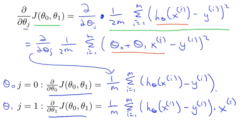
h_\theta(x)=\theta_0+\theta_1x \\ J(\theta_0,\theta_1)=\frac{1}{2m}\sum_{i=1}^m(h(x^i)-y^i)^2
h θ ( x ) = θ 0 + θ 1 x J ( θ 0 , θ 1 ) = 2 m 1 i = 1 ∑ m ( h ( x i ) − y i ) 2
(
x
i
,
y
i
)
(x^i,y^i)
( x i , y i )
i
=
1
,
2
,
.
.
.
,
m
i=1,2,...,m
i = 1 , 2 , . . . , m
x
x
x
y
y
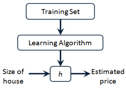
y 假设函数h (hypothesis):是一个从输入
x
x
x
y
y
y
h
(
x
)
=
θ
0
+
θ
1
x
h(x)=\theta_0+\theta_1x
h ( x ) = θ 0 + θ 1 x
θ
0
\theta_0
θ 0
θ
1
\theta_1
θ 1
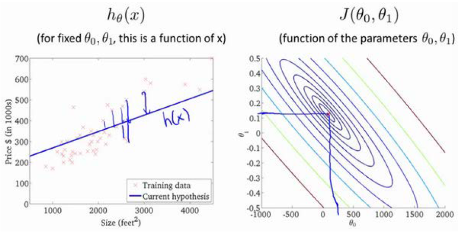
代价函数 (cost function)
J
(
θ
)
J(\theta)
J ( θ )
J
(
θ
0
,
θ
1
)
=
1
2
m
∑
i
=
1
m
(
h
(
x
i
)
−
y
i
)
2
,
m
为
训
练
样
本
的
数
量
。
J(\theta_0,\theta_1)=\frac{1}{2m}\sum_{i=1}^m(h(x^i)-y^i)^2,m为训练样本的数量。
J ( θ 0 , θ 1 ) = 2 m 1 i = 1 ∑ m ( h ( x i ) − y i ) 2 , m 为 训 练 样 本 的 数 量 。
m
i
n
m
i
z
e
θ
0
,
θ
1
J
(
θ
0
,
θ
1
)
\underset {\theta_0,\theta_1} {minmize}J(\theta_0,\theta_1)
θ 0 , θ 1 m i n m i z e J ( θ 0 , θ 1 )
代价函数:
J
(
θ
0
,
θ
1
)
J(\theta_0,\theta_1)
J ( θ 0 , θ 1 )
J
(
θ
0
,
θ
1
,
θ
2
,
.
.
.
,
θ
n
)
J(\theta_0,\theta_1,\theta_2,...,\theta_n)
J ( θ 0 , θ 1 , θ 2 , . . . , θ n )
m
i
n
θ
0
,
θ
1
J
(
θ
0
,
θ
1
)
\underset {\theta_0,\theta_1} {min}J(\theta_0,\theta_1)
θ 0 , θ 1 m i n J ( θ 0 , θ 1 )
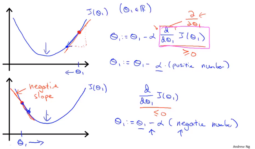
θ
0
,
θ
1
\theta_0,\theta_1
θ 0 , θ 1
θ
j
=
θ
j
−
α
∂
∂
θ
j
J
(
θ
0
,
θ
1
)
\theta_j=\theta_j-\alpha\frac{\partial}{\partial\theta_j}J(\theta_0,\theta_1)
θ j = θ j − α ∂ θ j ∂ J ( θ 0 , θ 1 )
α
\alpha
α
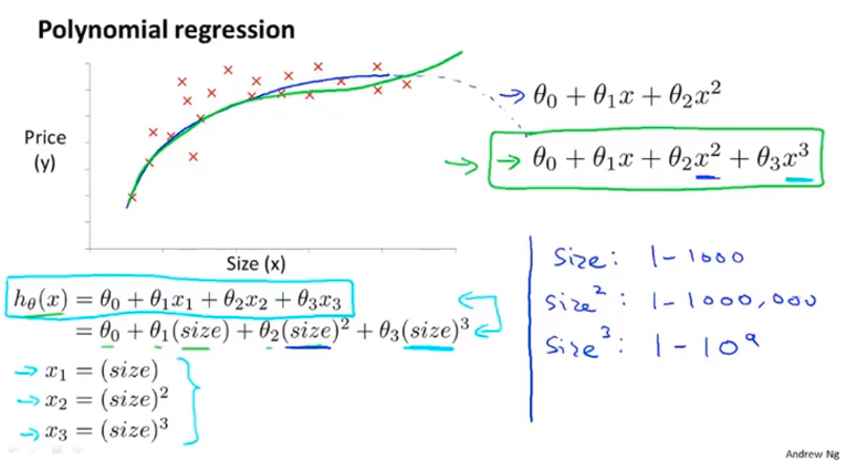
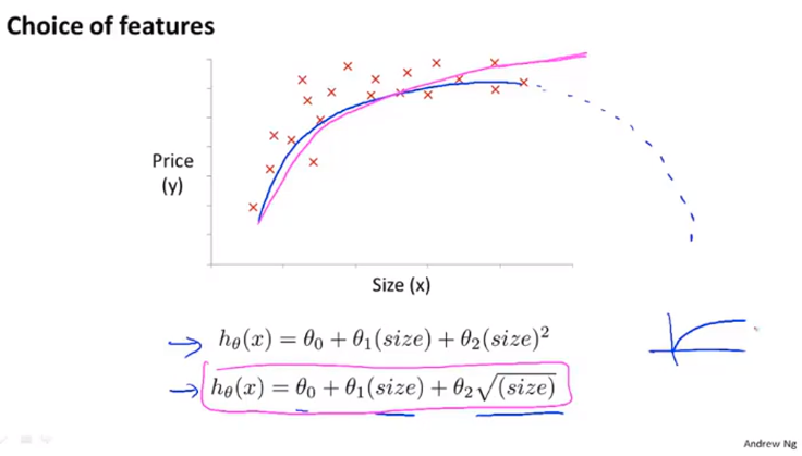
假设函数 :
h
θ
(
x
)
=
θ
0
+
θ
1
x
1
+
θ
2
x
2
+
⋯
+
θ
n
x
n
h_\theta(x)=\theta_0+\theta_1x_1+\theta_2x_2+\dots+\theta_nx_n
h θ ( x ) = θ 0 + θ 1 x 1 + θ 2 x 2 + ⋯ + θ n x n
x
0
=
1
x_0=1
x 0 = 1
x
=
[
x
0
,
x
1
,
x
2
,
…
,
x
n
]
T
,
x
∈
R
n
+
1
x=[x_0,x_1,x_2,\dots,x_n]^T,x\in\R^{n+1}
x = [ x 0 , x 1 , x 2 , … , x n ] T , x ∈ R n + 1
θ
=
[
θ
0
,
θ
1
,
θ
2
,
…
,
θ
n
]
T
,
θ
∈
R
n
+
1
\theta=[\theta_0,\theta_1,\theta_2,\dots,\theta_n]^T,\theta\in\R^{n+1}
θ = [ θ 0 , θ 1 , θ 2 , … , θ n ] T , θ ∈ R n + 1
h
θ
(
x
)
=
θ
T
x
h_\theta(x)=\theta^Tx
h θ ( x ) = θ T x 代价函数 :
J
(
θ
)
=
1
2
m
∑
i
=
1
m
(
h
θ
(
x
(
i
)
)
−
y
(
i
)
)
2
J(\theta)=\frac{1}{2m}\sum_{i=1}^{m}(h_\theta(x^{(i)})-y^{(i)})^2
J ( θ ) = 2 m 1 i = 1 ∑ m ( h θ ( x ( i ) ) − y ( i ) ) 2 梯度下降更新公式 :
θ
j
:
=
θ
j
−
α
∂
∂
θ
j
J
(
θ
)
,
j
=
0
,
1
,
…
,
n
\theta_j:=\theta_j-\alpha\frac{\partial}{\partial\theta_j}J(\theta),\ j=0,1,\dots,n
θ j : = θ j − α ∂ θ j ∂ J ( θ ) , j = 0 , 1 , … , n
θ
j
:
=
θ
j
−
α
1
m
∑
i
=
1
m
(
h
θ
(
x
(
i
)
)
−
y
(
i
)
)
x
j
(
i
)
,
j
=
0
,
1
,
…
,
n
\theta_j:=\theta_j-\alpha\frac{1}{m}\sum_{i=1}^{m}(h_\theta(x^{(i)})-y^{(i)})x_j^{(i)},\ j=0,1,\dots,n
θ j : = θ j − α m 1 i = 1 ∑ m ( h θ ( x ( i ) ) − y ( i ) ) x j ( i ) , j = 0 , 1 , … , n 可以通过for循环更新
θ
\theta
θ
θ
\theta
θ
θ
=
θ
−
α
m
X
T
(
X
θ
−
y
)
\theta=\theta-\frac{\alpha}{m}X^T(X\theta-y)
θ = θ − m α X T ( X θ − y )
目的:保证特征处于相似的尺度上,有利于加快梯度下降算法运行速度,加快收敛到全局最小值Mean normalization :
x
i
=
x
i
−
μ
σ
x_i=\frac{x_i-\mu}{\sigma}
x i = σ x i − μ
μ
\mu
μ
σ
\sigma
σ max-min:
x
i
=
x
i
−
m
i
n
m
a
x
−
m
i
n
x_i=\frac{x_i-min}{max-min}
x i = m a x − m i n x i − m i n
梯度下降更新公式 :
θ
j
:
=
θ
j
−
α
∂
∂
θ
j
J
(
θ
)
,
\theta_j:=\theta_j-\alpha\frac{\partial}{\partial\theta_j}J(\theta),
θ j : = θ j − α ∂ θ j ∂ J ( θ ) ,
“debugging”:如何确保梯度下降正确运行;
如何正确选择学习率。
如果
α
\alpha
α
如果
α
\alpha
α
J
(
θ
)
J(\theta)
J ( θ )
J
(
θ
)
J(\theta)
J ( θ )
choose
α
\alpha
α
…
,
0.001
,
0.003
,
0.01
,
0.03
,
0.1
,
0.3
,
1
,
…
\dots,0.001,0.003,0.01,0.03,0.1,0.3,1,\dots
… , 0 . 0 0 1 , 0 . 0 0 3 , 0 . 0 1 , 0 . 0 3 , 0 . 1 , 0 . 3 , 1 , …
寻找一个合适的较小值和较大值,保证结果和速度的同时选取较大的值,或者稍小的合理值。
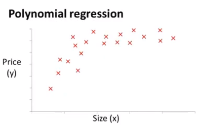
举例:房价预测问题
x
1
x_1
x 1
x
2
x_2
x 2
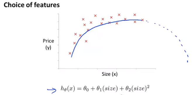
h
θ
(
x
)
=
θ
0
+
θ
1
x
1
+
θ
2
x
2
h_\theta(x)=\theta_0+\theta_1x_1+\theta_2x_2
h θ ( x ) = θ 0 + θ 1 x 1 + θ 2 x 2
x
=
x
1
∗
x
2
x=x_1*x_2
x = x 1 ∗ x 2
h
θ
(
x
)
=
θ
0
+
θ
1
x
h_\theta(x)=\theta_0+\theta_1x
h θ ( x ) = θ 0 + θ 1 x
代价函数:
J
(
θ
)
=
1
2
m
∑
i
=
1
m
(
h
θ
(
x
(
i
)
)
−
y
(
i
)
)
2
J(\theta)=\frac{1}{2m}\sum_{i=1}^{m}(h_\theta(x^{(i)})-y^{(i)})^2
J ( θ ) = 2 m 1 i = 1 ∑ m ( h θ ( x ( i ) ) − y ( i ) ) 2
J
(
θ
)
J(\theta)
J ( θ )
θ
=
(
X
T
X
)
−
1
X
T
y
\theta=(X^TX)^{-1}X^Ty
θ = ( X T X ) − 1 X T y
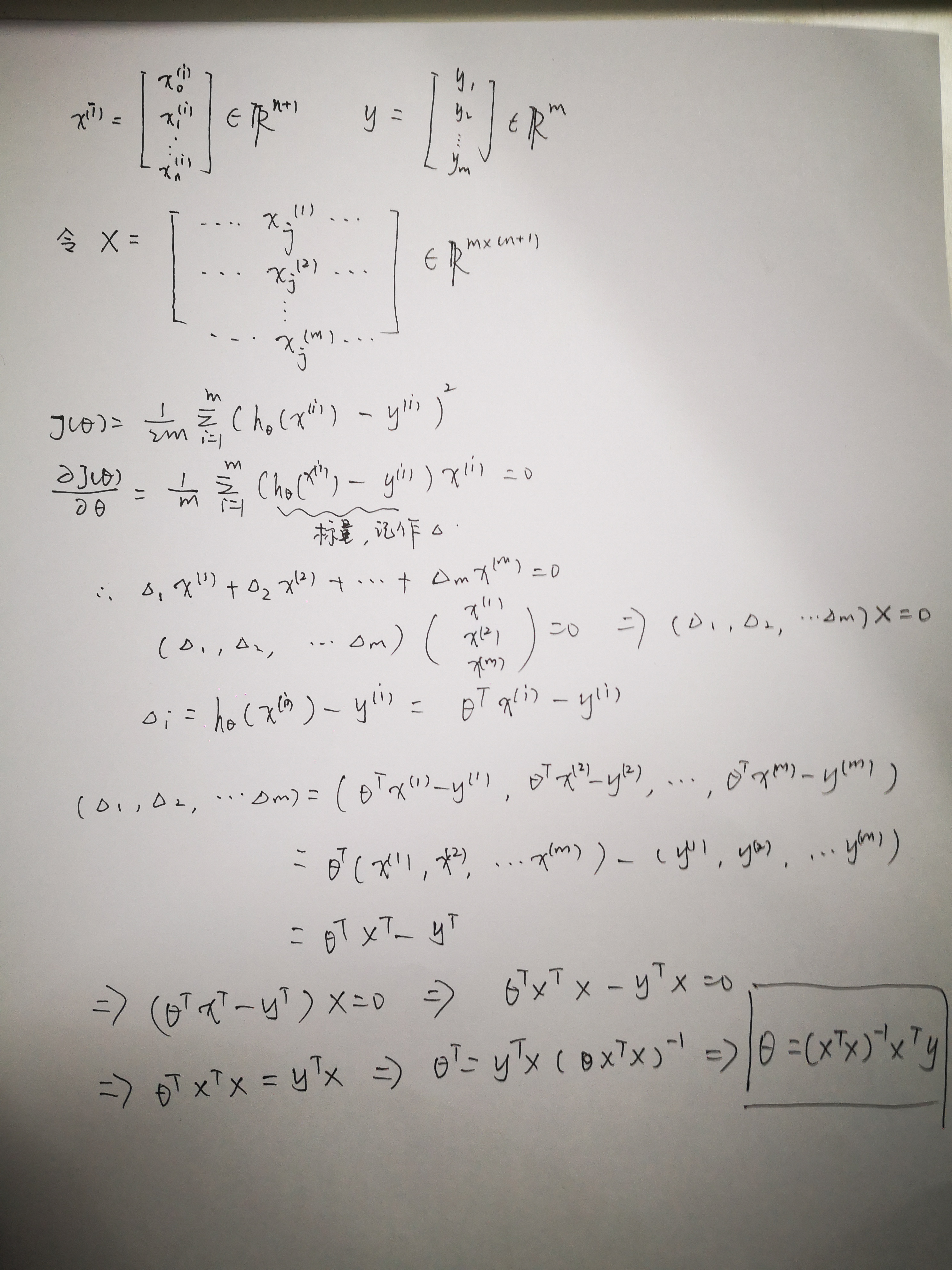
x
(
i
)
=
(
x
0
(
i
)
x
1
(
i
)
⋮
x
n
(
i
)
)
∈
R
n
+
1
,
y
=
(
y
1
y
2
⋮
y
m
)
∈
R
m
x^{(i)}=\begin{pmatrix}x_0^{(i)}\\x_1^{(i)}\\\vdots\\x_n^{(i)}\\\end{pmatrix}\in\R^{n+1},y=\begin{pmatrix}y_1\\y_2\\\vdots\\y_m\\\end{pmatrix}\in\R^m
x ( i ) = ⎝ ⎜ ⎜ ⎜ ⎜ ⎛ x 0 ( i ) x 1 ( i ) ⋮ x n ( i ) ⎠ ⎟ ⎟ ⎟ ⎟ ⎞ ∈ R n + 1 , y = ⎝ ⎜ ⎜ ⎜ ⎛ y 1 y 2 ⋮ y m ⎠ ⎟ ⎟ ⎟ ⎞ ∈ R m
X
=
(
1
x
1
(
1
)
⋯
x
j
(
1
)
⋯
x
n
(
1
)
1
x
1
(
2
)
⋯
x
j
(
2
)
⋯
x
n
(
2
)
⋮
⋮
⋱
⋮
⋱
⋮
1
x
1
(
m
)
⋯
x
j
(
m
)
⋯
x
n
(
m
)
)
=
(
(
x
(
1
)
)
T
(
x
(
2
)
)
T
⋮
(
x
(
m
)
)
T
)
∈
R
m
×
(
n
+
1
)
X=\begin{pmatrix} 1 & x_1^{(1)} & \cdots & x_j^{(1)} & \cdots & x_n^{(1)} \\ 1 & x_1^{(2)} & \cdots & x_j^{(2)} & \cdots & x_n^{(2)} \\ \vdots & \vdots & \ddots & \vdots & \ddots & \vdots \\ 1 & x_1^{(m)} & \cdots & x_j^{(m)} & \cdots & x_n^{(m)} \\ \end{pmatrix} =\begin{pmatrix} (x^{(1)})^T\\(x^{(2)})^T\\\vdots\\(x^{(m)})^T \end{pmatrix}\in\R^{m×(n+1)}
X = ⎝ ⎜ ⎜ ⎜ ⎜ ⎛ 1 1 ⋮ 1 x 1 ( 1 ) x 1 ( 2 ) ⋮ x 1 ( m ) ⋯ ⋯ ⋱ ⋯ x j ( 1 ) x j ( 2 ) ⋮ x j ( m ) ⋯ ⋯ ⋱ ⋯ x n ( 1 ) x n ( 2 ) ⋮ x n ( m ) ⎠ ⎟ ⎟ ⎟ ⎟ ⎞ = ⎝ ⎜ ⎜ ⎜ ⎛ ( x ( 1 ) ) T ( x ( 2 ) ) T ⋮ ( x ( m ) ) T ⎠ ⎟ ⎟ ⎟ ⎞ ∈ R m × ( n + 1 )
∂
∂
θ
J
(
θ
)
=
1
m
∑
i
=
1
m
(
h
θ
(
x
(
i
)
)
−
y
(
i
)
)
x
(
i
)
=
0
\frac{\partial}{\partial\theta}J(\theta)=\frac{1}{m}\sum_{i=1}^{m}(h_\theta(x^{(i)})-y^{(i)})x^{(i)}=0
∂ θ ∂ J ( θ ) = m 1 ∑ i = 1 m ( h θ ( x ( i ) ) − y ( i ) ) x ( i ) = 0
θ
=
(
X
T
X
)
−
1
X
T
y
\theta = (X^TX)^{-1}X^Ty
θ = ( X T X ) − 1 X T y
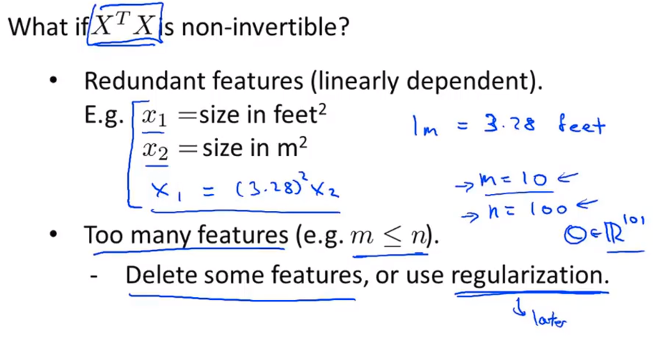
X
T
X
X^TX
X T X 梯度下降算法 :需要选择学习速率
α
\alpha
α 正规方程: 无需选择参数;无需迭代;需要计算
(
X
T
X
)
−
1
(X^TX)^{-1}
( X T X ) − 1
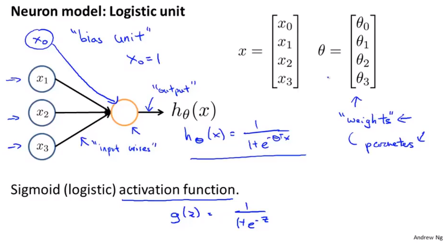
逻辑回归模型:
h
θ
(
x
)
,
h_\theta(x),
h θ ( x ) ,
0
≤
h
θ
(
x
)
≤
1
0 \leq h_\theta(x) \leq 1
0 ≤ h θ ( x ) ≤ 1
h
θ
(
x
)
=
g
(
θ
T
x
)
\ h_\theta(x)\ =g(\theta^Tx)
h θ ( x ) = g ( θ T x )
θ
T
x
\theta^Tx
θ T x
g
(
⋅
)
g(\cdot)
g ( ⋅ )
h
θ
(
x
)
=
1
1
+
e
−
θ
T
x
h_\theta(x)=\frac{1}{1+e^{-\theta^Tx}}
h θ ( x ) = 1 + e − θ T x 1
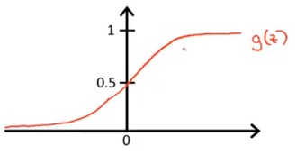
g
(
z
)
=
1
1
+
e
−
z
g(z)=\frac{1}{1+e^{-z}}
g ( z ) = 1 + e − z 1 Sigmod函数 ,也叫作Logistic函数 。
{
h
θ
(
x
)
≥
0.5
,
y
=
1
h
θ
(
x
)
<
0.5
,
y
=
0
\begin{cases} h_\theta(x) \geq 0.5,y=1 \\ h_\theta(x) < 0.5,y=0 \end{cases}
{ h θ ( x ) ≥ 0 . 5 , y = 1 h θ ( x ) < 0 . 5 , y = 0
h
θ
(
x
)
=
p
{
y
=
1
∣
x
,
θ
}
h_\theta(x)=p\{y=1|x,\theta\}
h θ ( x ) = p { y = 1 ∣ x , θ }
predict:y=1
,
if
h
θ
(
x
)
≥
0.5
\text {predict:y=1},\text {if }h_\theta(x) \geq 0.5
predict : y=1 , if h θ ( x ) ≥ 0 . 5
predict:y=0
,
if
h
θ
(
x
)
<
0.5
\text {predict:y=0},\text {if }h_\theta(x) < 0.5
predict : y=0 , if h θ ( x ) < 0 . 5
h
θ
(
x
)
≥
0.5
→
z
≥
0
→
θ
T
x
≥
0
h_\theta(x) \geq 0.5\quad \to\quad z\geq0 \quad \to\quad \theta^Tx\geq0
h θ ( x ) ≥ 0 . 5 → z ≥ 0 → θ T x ≥ 0
h
θ
(
x
)
<
0.5
→
z
<
0
→
θ
T
x
<
0
h_\theta(x) < 0.5\quad \to\quad z<0 \quad \to\quad \theta^Tx<0
h θ ( x ) < 0 . 5 → z < 0 → θ T x < 0
θ
T
x
=
0
\theta^Tx=0
θ T x = 0 决策边界 。
假设表示定义的:
h
θ
(
x
)
=
p
{
y
=
1
∣
x
,
θ
}
h_\theta(x)=p\{y=1|x,\theta\}
h θ ( x ) = p { y = 1 ∣ x , θ } 极大似然 的思想:
θ
=
a
r
g
m
a
x
θ
∏
i
=
1
m
p
{
y
i
=
1
∣
x
,
θ
}
y
i
p
{
y
i
=
0
∣
x
,
θ
}
1
−
y
i
=
a
r
g
m
a
x
θ
∏
i
=
1
m
p
{
y
i
=
1
∣
x
,
θ
}
y
i
(
1
−
p
{
y
i
=
1
∣
x
,
θ
}
)
1
−
y
i
\begin{array}{} \theta=\underset{\theta}{argmax}\prod_{i=1}^{m}p\{y_i=1|x,\theta\}^{y_i}p\{y_i=0|x,\theta\}^{1-y_i}\\ = \underset{\theta}{argmax}\prod_{i=1}^{m}p\{y_i=1|x,\theta\}^{y_i}(1-p\{y_i=1|x,\theta\})^{1-y_i} \end{array}{}
θ = θ a r g m a x ∏ i = 1 m p { y i = 1 ∣ x , θ } y i p { y i = 0 ∣ x , θ } 1 − y i = θ a r g m a x ∏ i = 1 m p { y i = 1 ∣ x , θ } y i ( 1 − p { y i = 1 ∣ x , θ } ) 1 − y i
Γ
=
∏
i
=
1
m
p
{
y
i
=
1
∣
x
,
θ
}
y
i
(
1
−
p
{
y
i
=
1
∣
x
,
θ
}
)
1
−
y
i
\Gamma=\prod_{i=1}^{m}p\{y_i=1|x,\theta\}^{y_i}(1-p\{y_i=1|x,\theta\})^{1-y_i}
Γ = ∏ i = 1 m p { y i = 1 ∣ x , θ } y i ( 1 − p { y i = 1 ∣ x , θ } ) 1 − y i
log
(
Γ
)
=
∑
i
=
1
m
y
i
log
(
h
θ
(
x
)
)
+
(
1
−
y
i
)
(
1
−
log
(
h
θ
(
x
)
)
)
\log(\Gamma)=\sum_{i=1}^my_i\log(h_\theta(x))+(1-y_i)(1-\log(h_\theta(x)))
log ( Γ ) = i = 1 ∑ m y i log ( h θ ( x ) ) + ( 1 − y i ) ( 1 − log ( h θ ( x ) ) )
θ
=
a
r
g
m
a
x
θ
log
(
Γ
)
=
a
r
g
m
a
x
θ
∑
i
=
1
m
y
i
log
(
h
θ
(
x
)
)
+
(
1
−
y
i
)
(
1
−
log
(
h
θ
(
x
)
)
)
\theta = \underset{\theta}{argmax}\log(\Gamma)\\=\underset{\theta}{argmax}\sum_{i=1}^my_i\log(h_\theta(x))+(1-y_i)(1-\log(h_\theta(x)))
θ = θ a r g m a x log ( Γ ) = θ a r g m a x i = 1 ∑ m y i log ( h θ ( x ) ) + ( 1 − y i ) ( 1 − log ( h θ ( x ) ) )
c
o
s
t
(
h
θ
(
x
)
,
y
i
)
=
−
y
i
log
(
h
θ
(
x
)
)
−
(
1
−
y
i
)
(
1
−
log
(
h
θ
(
x
)
)
)
cost(h_\theta(x),y_i)=-y_i\log(h_\theta(x))-(1-y_i)(1-\log(h_\theta(x)))
c o s t ( h θ ( x ) , y i ) = − y i log ( h θ ( x ) ) − ( 1 − y i ) ( 1 − log ( h θ ( x ) ) )
θ
=
a
r
g
m
a
x
θ
∑
i
=
1
m
c
o
s
t
(
h
θ
(
x
)
,
y
i
)
\theta= \underset{\theta}{argmax}\sum_{i=1}^mcost(h_\theta(x),y_i)
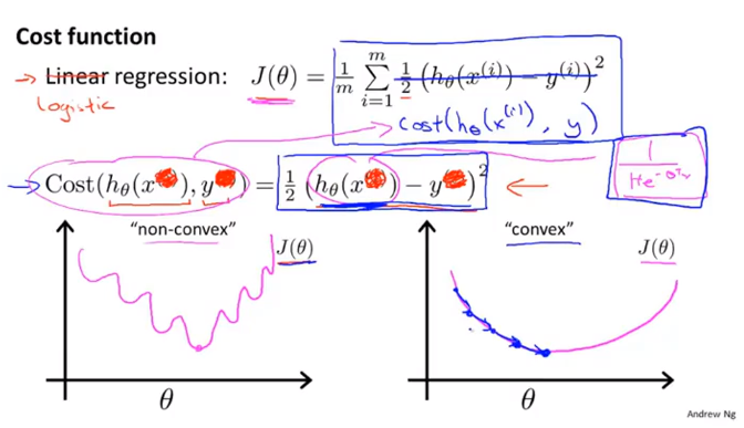
θ = θ a r g m a x i = 1 ∑ m c o s t ( h θ ( x ) , y i ) 注意 :线性回归的
c
o
s
t
(
h
θ
(
x
)
,
y
i
)
=
(
h
θ
(
x
)
−
y
i
)
2
cost(h_\theta(x),y_i)=(h_\theta(x)-y_i)^2
c o s t ( h θ ( x ) , y i ) = ( h θ ( x ) − y i ) 2
c
o
s
t
(
h
θ
(
x
)
,
y
i
)
=
−
y
i
log
(
h
θ
(
x
)
)
−
(
1
−
y
i
)
(
1
−
log
(
h
θ
(
x
)
)
)
cost(h_\theta(x),y_i)=-y_i\log(h_\theta(x))-(1-y_i)(1-\log(h_\theta(x)))
c o s t ( h θ ( x ) , y i ) = − y i log ( h θ ( x ) ) − ( 1 − y i ) ( 1 − log ( h θ ( x ) ) )
c
o
s
t
(
h
θ
(
x
)
,
y
i
)
=
{
−
y
i
log
(
h
θ
(
x
)
)
,
if
y
i
=
1
−
(
1
−
y
i
)
(
1
−
log
(
h
θ
(
x
)
)
)
,
if
y
i
=
0
cost(h_\theta(x),y_i)=\begin{cases} -y_i\log(h_\theta(x)),\quad \quad \quad \quad\quad\text{if $y_i=1$} \\-(1-y_i)(1-\log(h_\theta(x))),\text{if $y_i=0$}\end{cases}
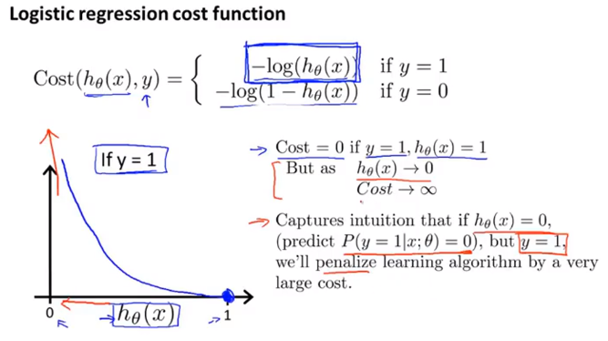
c o s t ( h θ ( x ) , y i ) = { − y i log ( h θ ( x ) ) , if y i = 1 − ( 1 − y i ) ( 1 − log ( h θ ( x ) ) ) , if y i = 0 逻辑回归代价函数 :
J
(
θ
)
=
1
m
∑
i
=
1
m
c
o
s
t
(
h
θ
(
x
(
i
)
)
,
y
(
i
)
)
=
−
1
m
∑
i
=
1
m
(
y
(
i
)
log
(
h
θ
(
x
(
i
)
)
)
+
(
1
−
y
(
i
)
)
log
(
1
−
h
θ
(
x
(
i
)
)
)
)
J(\theta)=\frac{1}{m}\sum_{i=1}^{m}cost(h_\theta(x^{(i)}),y^{(i)})\\=-\frac{1}{m}\sum_{i=1}^{m}(y^{(i)}\log(h_\theta(x^{(i)}))+(1-y^{(i)})\log(1-h_\theta(x^{(i)})))
J ( θ ) = m 1 i = 1 ∑ m c o s t ( h θ ( x ( i ) ) , y ( i ) ) = − m 1 i = 1 ∑ m ( y ( i ) log ( h θ ( x ( i ) ) ) + ( 1 − y ( i ) ) log ( 1 − h θ ( x ( i ) ) ) ) 拟合参数 :
min
θ
J
(
θ
)
\underset{\theta}{\min}J(\theta)
θ min J ( θ ) 梯度下降法 :
∂
∂
θ
j
J
(
θ
)
=
1
m
∑
i
=
1
m
(
h
θ
(
x
(
i
)
)
−
y
(
i
)
)
x
j
(
i
)
\frac{\partial}{\partial\theta_j}J(\theta)=\frac{1}{m}\sum_{i=1}^{m}(h_\theta(x^{(i)})-y^{(i)})x_j^{(i)}
∂ θ j ∂ J ( θ ) = m 1 i = 1 ∑ m ( h θ ( x ( i ) ) − y ( i ) ) x j ( i )
θ
j
:
=
θ
j
−
α
∂
∂
θ
j
J
(
θ
)
=
θ
j
−
α
m
∑
i
=
1
m
(
h
θ
(
x
(
i
)
)
−
y
(
i
)
)
x
j
(
i
)
\theta_j:=\theta_j-\alpha\frac{\partial}{\partial\theta_j}J(\theta)=\theta_j-\frac{\alpha}{m}\sum_{i=1}^{m}(h_\theta(x^{(i)})-y^{(i)})x_j^{(i)}
θ j : = θ j − α ∂ θ j ∂ J ( θ ) = θ j − m α i = 1 ∑ m ( h θ ( x ( i ) ) − y ( i ) ) x j ( i ) 高级优化算法 :
共轭梯度算法
BFGS
L-BFGS
α
\alpha
α
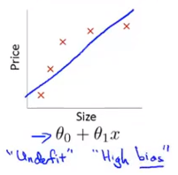
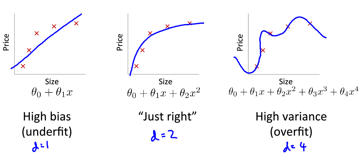
欠拟合,高偏差 :说明没有很好的拟合训练数据解决办法 :增加特征,如增加多项式
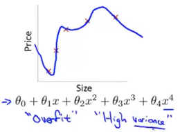
过拟合,高方差 :拟合训练数据过于完美,
J
(
θ
)
≈
0
J(\theta)\approx0
J ( θ ) ≈ 0 解决办法 :
减少特征个数
正规化
θ
j
\theta_j
θ j
对
θ
j
\theta_j
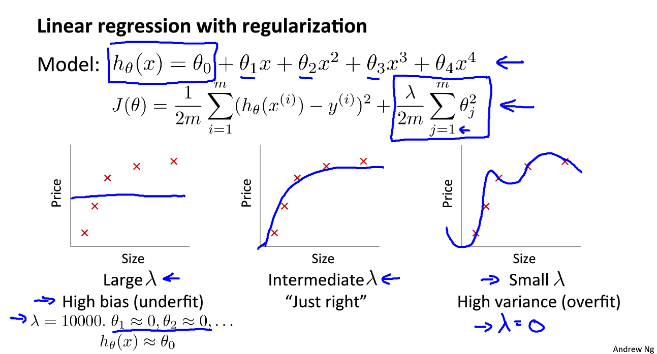
θ j 线性回归代价函数 :
J
(
θ
)
=
1
2
m
[
∑
i
=
1
m
(
h
θ
(
x
(
i
)
)
−
y
(
i
)
)
2
+
λ
∑
j
=
1
m
θ
j
2
]
J(\theta)=\frac{1}{2m}\left[ \sum_{i=1}^{m}(h_\theta(x^{(i)})-y^{(i)})^2+\lambda\sum_{j=1}^m\theta_j^2\right]
J ( θ ) = 2 m 1 [ i = 1 ∑ m ( h θ ( x ( i ) ) − y ( i ) ) 2 + λ j = 1 ∑ m θ j 2 ] 逻辑回归代价函数 :
J
(
θ
)
=
−
1
m
∑
i
=
1
m
(
y
(
i
)
log
(
h
θ
(
x
(
i
)
)
)
+
(
1
−
y
(
i
)
)
log
(
1
−
h
θ
(
x
(
i
)
)
)
)
+
λ
2
m
∑
j
=
1
m
θ
j
2
J(\theta)=-\frac{1}{m}\sum_{i=1}^{m}(y^{(i)}\log(h_\theta(x^{(i)}))+(1-y^{(i)})\log(1-h_\theta(x^{(i)})))+\frac{\lambda}{2m}\sum_{j=1}^{m}\theta_j^2
J ( θ ) = − m 1 i = 1 ∑ m ( y ( i ) log ( h θ ( x ( i ) ) ) + ( 1 − y ( i ) ) log ( 1 − h θ ( x ( i ) ) ) ) + 2 m λ j = 1 ∑ m θ j 2 拟合参数 :
min
θ
J
(
θ
)
\underset{\theta}{\min}J(\theta)
θ min J ( θ )
min
θ
J
(
θ
)
\underset{\theta}{\min}J(\theta)
θ min J ( θ )
梯度下降算法:
θ
0
:
=
θ
0
−
α
1
m
∑
i
=
1
m
(
h
θ
(
x
(
i
)
)
−
y
(
i
)
)
x
0
(
i
)
\theta_0:= \theta_0-\alpha\frac{1}{m}\sum_{i=1}^m(h_\theta(x^{(i)})-y^{(i)})x_0^{(i)}
θ 0 : = θ 0 − α m 1 i = 1 ∑ m ( h θ ( x ( i ) ) − y ( i ) ) x 0 ( i )
θ
j
:
=
θ
j
−
α
1
m
[
∑
i
=
1
m
(
h
θ
(
x
(
i
)
)
−
y
(
i
)
)
x
0
(
i
)
+
λ
θ
j
]
\theta_j:= \theta_j-\alpha\frac{1}{m}\left[\sum_{i=1}^m(h_\theta(x^{(i)})-y^{(i)})x_0^{(i)}+\lambda\theta_j\right]
θ j : = θ j − α m 1 [ i = 1 ∑ m ( h θ ( x ( i ) ) − y ( i ) ) x 0 ( i ) + λ θ j ]
\quad\quad\quad\;
θ
0
:
=
θ
0
−
α
1
m
∑
i
=
1
m
(
h
θ
(
x
(
i
)
)
−
y
(
i
)
)
x
0
(
i
)
\theta_0:= \theta_0-\alpha\frac{1}{m}\sum_{i=1}^m(h_\theta(x^{(i)})-y^{(i)})x_0^{(i)}
θ 0 : = θ 0 − α m 1 i = 1 ∑ m ( h θ ( x ( i ) ) − y ( i ) ) x 0 ( i )
θ
j
:
=
θ
j
(
1
−
α
1
m
)
−
α
1
m
∑
i
=
1
m
(
h
θ
(
x
(
i
)
)
−
y
(
i
)
)
x
0
(
i
)
\theta_j:= \theta_j(1-\alpha\frac{1}{m})-\alpha\frac{1}{m}\sum_{i=1}^m(h_\theta(x^{(i)})-y^{(i)})x_0^{(i)}
θ j : = θ j ( 1 − α m 1 ) − α m 1 i = 1 ∑ m ( h θ ( x ( i ) ) − y ( i ) ) x 0 ( i )
\quad\quad\quad\;
正规方程 :
m
≤
n
(
e
x
a
m
p
l
e
s
≤
f
e
a
t
u
r
e
s
)
m\leq n(examples\leq features)
m ≤ n ( e x a m p l e s ≤ f e a t u r e s )
θ
=
(
X
T
X
)
−
1
X
T
y
\theta=(X^TX)^{-1}X^Ty
θ = ( X T X ) − 1 X T y
λ
>
0
\lambda>0
λ > 0
θ
=
(
X
T
X
+
λ
[
0
1
1
⋱
1
]
⎵
(
n
+
1
)
×
(
n
+
1
)
)
−
1
X
T
y
\theta=\left(X^TX+\lambda\underbrace{ \begin{bmatrix}0\\ &1\\ &&1\\ &&& \ddots \\&&&&1\end{bmatrix}}_{(n+1)\times(n+1)}\right)^{-1}X^Ty
θ = ⎝ ⎜ ⎜ ⎜ ⎜ ⎜ ⎜ ⎜ ⎜ ⎜ ⎛ X T X + λ ( n + 1 ) × ( n + 1 )
⎣ ⎢ ⎢ ⎢ ⎢ ⎡ 0 1 1 ⋱ 1 ⎦ ⎥ ⎥ ⎥ ⎥ ⎤ ⎠ ⎟ ⎟ ⎟ ⎟ ⎟ ⎟ ⎟ ⎟ ⎟ ⎞ − 1 X T y
λ
>
0
\lambda>0
λ > 0
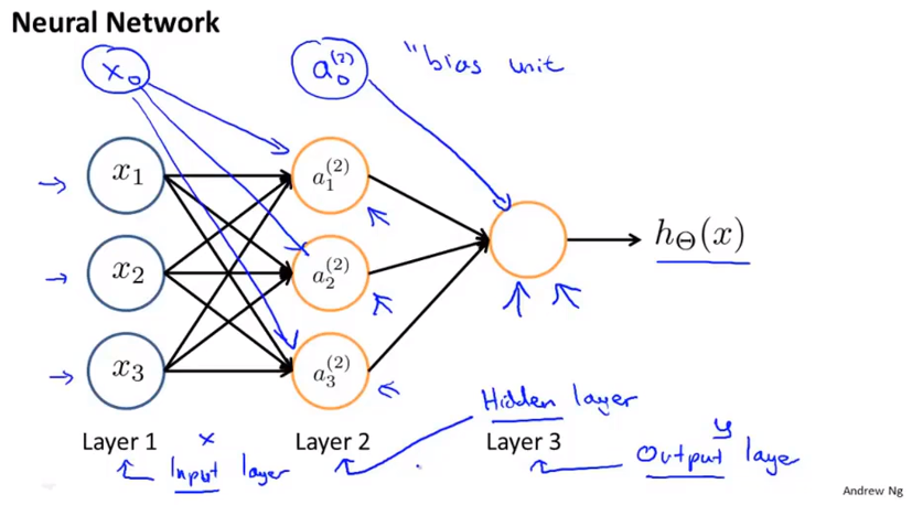
a
i
(
j
)
a^{(j)}_i
a i ( j )
j
j
j
i
i
i i in layer j ”)
Θ
(
j
)
\Theta^{(j)}
Θ ( j )
j
j
j
u
n
i
t
s
units
u n i t s
s
j
s_j
s j
j
+
1
j+1
j + 1
u
n
i
t
s
units
u n i t s
s
j
+
1
s_{j+1}
s j + 1
s
j
+
1
×
(
s
j
+
1
)
s_{j+1}\times (s_j+1)
s j + 1 × ( s j + 1 )
a
1
(
2
)
=
g
(
Θ
10
(
1
)
x
0
+
Θ
11
(
1
)
x
1
+
Θ
12
(
1
)
x
2
+
Θ
13
(
1
)
x
3
)
a_1^{(2)}=g(\Theta_{10}^{(1)}x_0+\Theta_{11}^{(1)}x_1+\Theta_{12}^{(1)}x_2+\Theta_{13}^{(1)}x_3)
a 1 ( 2 ) = g ( Θ 1 0 ( 1 ) x 0 + Θ 1 1 ( 1 ) x 1 + Θ 1 2 ( 1 ) x 2 + Θ 1 3 ( 1 ) x 3 )
a
2
(
2
)
=
g
(
Θ
20
(
1
)
x
0
+
Θ
21
(
1
)
x
1
+
Θ
22
(
1
)
x
2
+
Θ
23
(
1
)
x
3
)
a_2^{(2)}=g(\Theta_{20}^{(1)}x_0+\Theta_{21}^{(1)}x_1+\Theta_{22}^{(1)}x_2+\Theta_{23}^{(1)}x_3)
a 2 ( 2 ) = g ( Θ 2 0 ( 1 ) x 0 + Θ 2 1 ( 1 ) x 1 + Θ 2 2 ( 1 ) x 2 + Θ 2 3 ( 1 ) x 3 )
a
3
(
2
)
=
g
(
Θ
30
(
1
)
x
0
+
Θ
31
(
1
)
x
1
+
Θ
32
(
1
)
x
2
+
Θ
33
(
1
)
x
3
)
a_3^{(2)}=g(\Theta_{30}^{(1)}x_0+\Theta_{31}^{(1)}x_1+\Theta_{32}^{(1)}x_2+\Theta_{33}^{(1)}x_3)
a 3 ( 2 ) = g ( Θ 3 0 ( 1 ) x 0 + Θ 3 1 ( 1 ) x 1 + Θ 3 2 ( 1 ) x 2 + Θ 3 3 ( 1 ) x 3 )
h
Θ
(
x
)
=
a
1
(
3
)
=
g
(
Θ
10
(
2
)
a
0
(
2
)
+
Θ
11
(
2
)
a
1
(
2
)
+
Θ
12
(
2
)
a
2
(
2
)
+
Θ
13
(
2
)
a
3
(
2
)
)
h_\Theta(x)=a_1^{(3)}=g(\Theta_{10}^{(2)}a_0^{(2)}+\Theta_{11}^{(2)}a_1^{(2)}+\Theta_{12}^{(2)}a_2 ^{(2)}+\Theta_{13}^{(2)}a_3^{(2)})
h Θ ( x ) = a 1 ( 3 ) = g ( Θ 1 0 ( 2 ) a 0 ( 2 ) + Θ 1 1 ( 2 ) a 1 ( 2 ) + Θ 1 2 ( 2 ) a 2 ( 2 ) + Θ 1 3 ( 2 ) a 3 ( 2 ) )
h
Θ
(
x
)
=
a
(
3
)
=
g
(
z
(
3
)
)
=
g
(
Θ
(
2
)
a
(
2
)
)
=
g
(
Θ
(
2
)
g
(
z
(
2
)
)
)
=
g
(
Θ
(
2
)
g
(
Θ
(
1
)
a
(
1
)
)
)
h_\Theta(x)=a^{(3)}=g(z^{(3)})=g(\Theta^{(2)}a^{(2)})=g(\Theta^{(2)}g(z^{(2)}))=g(\Theta^{(2)}g(\Theta^{(1)}a^{(1)}))
h Θ ( x ) = a ( 3 ) = g ( z ( 3 ) ) = g ( Θ ( 2 ) a ( 2 ) ) = g ( Θ ( 2 ) g ( z ( 2 ) ) ) = g ( Θ ( 2 ) g ( Θ ( 1 ) a ( 1 ) ) )
逻辑回归代价函数:
J
(
θ
)
=
−
1
m
∑
i
=
1
m
(
y
(
i
)
log
(
h
θ
(
x
(
i
)
)
)
+
(
1
−
y
(
i
)
)
log
(
1
−
h
θ
(
x
(
i
)
)
)
)
+
λ
2
m
∑
j
=
1
m
θ
j
2
J(\theta)=-\frac{1}{m}\sum_{i=1}^{m}(y^{(i)}\log(h_\theta(x^{(i)}))+(1-y^{(i)})\log(1-h_\theta(x^{(i)})))+\frac{\lambda}{2m}\sum_{j=1}^{m}\theta_j^2
J ( θ ) = − m 1 i = 1 ∑ m ( y ( i ) log ( h θ ( x ( i ) ) ) + ( 1 − y ( i ) ) log ( 1 − h θ ( x ( i ) ) ) ) + 2 m λ j = 1 ∑ m θ j 2 神经网络代价函数 :
J
(
θ
)
=
−
1
m
∑
i
=
1
m
∑
k
=
1
K
(
y
k
(
i
)
log
(
h
θ
(
x
(
i
)
)
)
k
+
(
1
−
y
k
(
i
)
)
log
(
1
−
h
θ
(
x
(
i
)
)
)
k
)
+
λ
2
m
∑
l
=
1
L
−
1
∑
j
=
1
m
∑
i
=
1
m
(
θ
j
i
l
)
2
J(\theta)=-\frac{1}{m}\sum_{i=1}^{m}\sum_{k=1}^{K}(y_k^{(i)}\log(h_\theta(x^{(i)}))_k+(1-y_k^{(i)})\log(1-h_\theta(x^{(i)}))_k)+\frac{\lambda}{2m}\sum_{l=1}^{L-1}\sum_{j=1}^{m}\sum_{i=1}^{m}(\theta_{ji}^{l})^2
J ( θ ) = − m 1 i = 1 ∑ m k = 1 ∑ K ( y k ( i ) log ( h θ ( x ( i ) ) ) k + ( 1 − y k ( i ) ) log ( 1 − h θ ( x ( i ) ) ) k ) + 2 m λ l = 1 ∑ L − 1 j = 1 ∑ m i = 1 ∑ m ( θ j i l ) 2 优化目标 :
min
Θ
J
(
Θ
)
\underset{\Theta}{\min} J(\Theta)
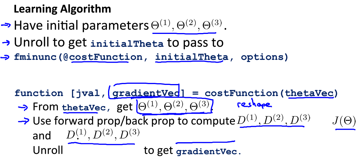
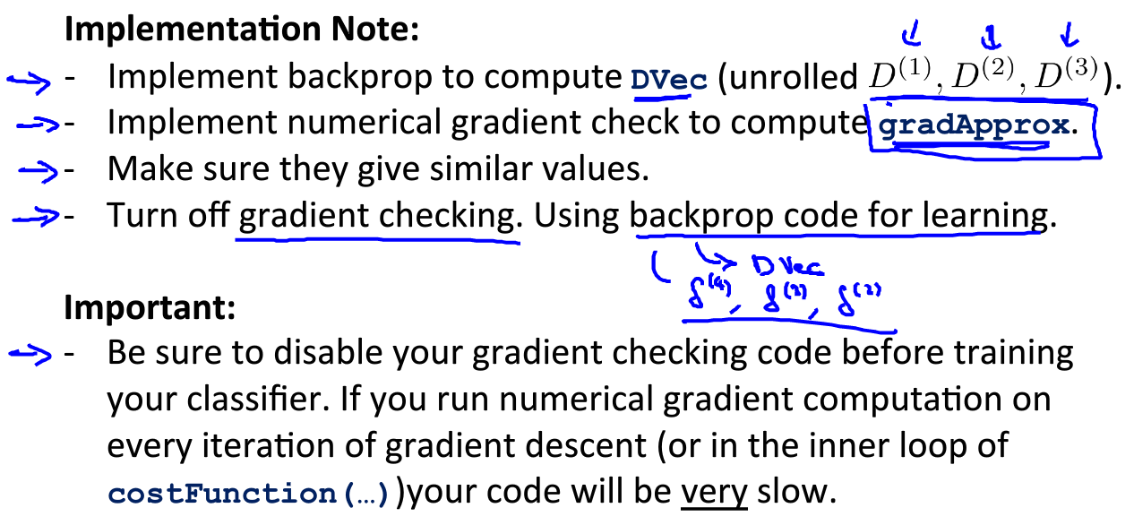
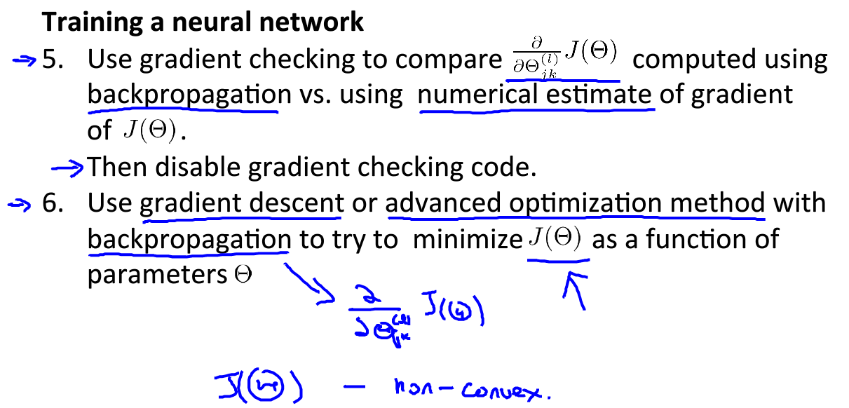
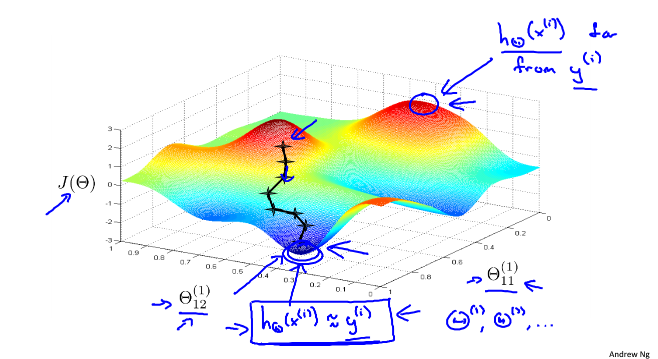
Θ min J ( Θ ) 需要计算 :
J
(
Θ
)
J(\Theta)
J ( Θ )
∂
∂
Θ
i
j
(
l
)
J
(
Θ
)
\frac{\partial}{\partial\Theta_{ij}^{(l)}}J(\Theta)
∂ Θ i j ( l ) ∂ J ( Θ )
Θ
i
j
(
l
)
∈
R
\Theta_{ij}^{(l)}\in\R
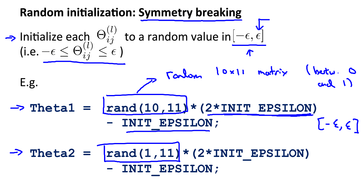
Θ i j ( l ) ∈ R
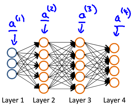
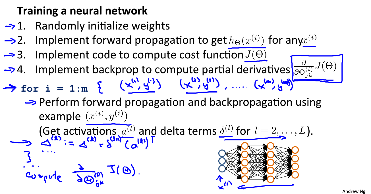
如图:前向传播 :
a
(
1
)
=
x
z
(
2
)
=
Θ
(
1
)
a
(
1
)
a
(
2
)
=
g
(
z
(
2
)
)
z
(
3
)
=
Θ
(
2
)
a
(
2
)
a
(
3
)
=
g
(
z
(
3
)
z
(
4
)
=
Θ
(
3
)
a
(
3
)
a
(
4
)
=
g
(
z
(
4
)
h
Θ
(
x
)
=
a
(
4
)
a^{(1)}=x \\ z^{(2)}=\Theta^{(1)}a^{(1)} \\ a^{(2)}=g(z^{(2)}) \\ z^{(3)}=\Theta^{(2)}a^{(2)} \\ a^{(3)}=g(z^{(3}) \\ z^{(4)}=\Theta^{(3)}a^{(3)} \\ a^{(4)}=g(z^{(4}) \\ h_{\Theta}(x)=a^{(4)}
a ( 1 ) = x z ( 2 ) = Θ ( 1 ) a ( 1 ) a ( 2 ) = g ( z ( 2 ) ) z ( 3 ) = Θ ( 2 ) a ( 2 ) a ( 3 ) = g ( z ( 3 ) z ( 4 ) = Θ ( 3 ) a ( 3 ) a ( 4 ) = g ( z ( 4 ) h Θ ( x ) = a ( 4 )
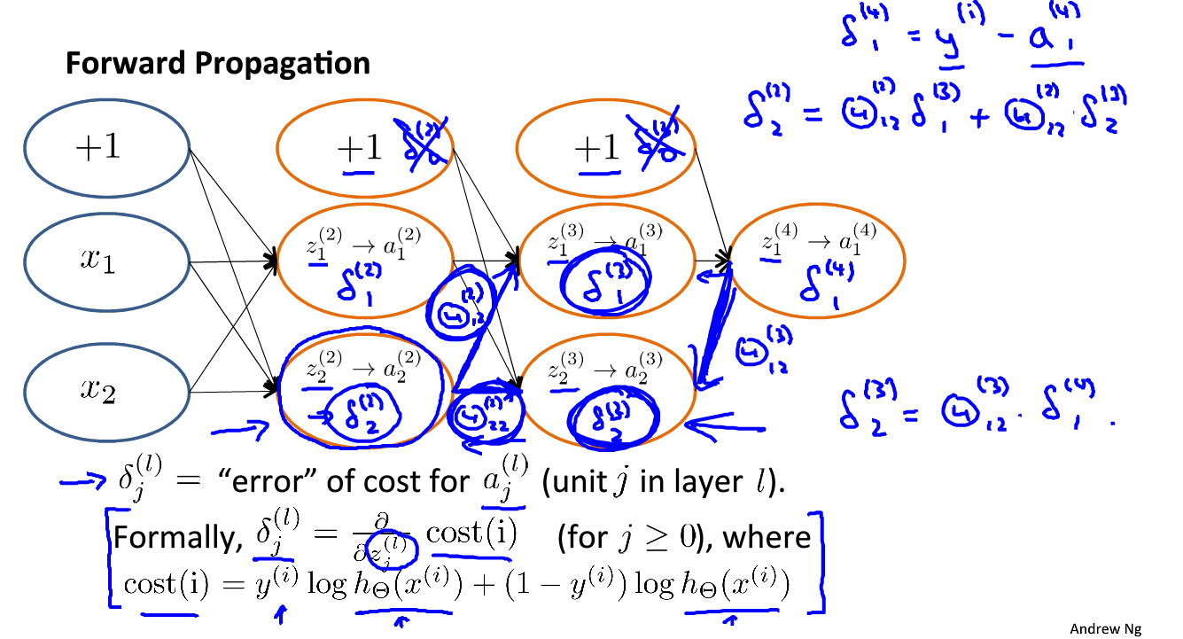
计算:
δ
j
(
l
)
\delta_j^{(l)}
δ j ( l )
l
l
l
j
j
j
δ
j
(
4
)
=
a
j
(
4
)
−
y
j
\delta_j^{(4)}=a_j^{(4)}-y_j
δ j ( 4 ) = a j ( 4 ) − y j
δ
(
4
)
=
a
(
4
)
−
y
\delta^{(4)}=a^{(4)}-y
δ ( 4 ) = a ( 4 ) − y
δ
(
l
)
、
δ
(
l
−
1
)
…
δ
(
2
)
\delta^{(l)}、\delta^{(l-1)}\dots \delta^{(2)}
δ ( l ) 、 δ ( l − 1 ) … δ ( 2 )
δ
(
3
)
=
(
Θ
(
3
)
)
T
δ
(
4
)
.
∗
g
′
(
z
(
3
)
)
,
g
′
(
z
(
3
)
)
=
a
(
3
)
.
∗
(
1
−
a
(
3
)
)
δ
(
2
)
=
(
Θ
(
2
)
)
T
δ
(
3
)
.
∗
g
′
(
z
(
2
)
)
,
g
′
(
z
(
2
)
)
=
a
(
2
)
.
∗
(
1
−
a
(
2
)
)
\delta^{(3)}=(\Theta^{(3)})^T\delta^{(4)}.*g\prime(z^{(3)}),\qquad g\prime(z^{(3)})=a^{(3)}.*(1-a^{(3)}) \\ \delta^{(2)}=(\Theta^{(2)})^T\delta^{(3)}.*g\prime(z^{(2)}),\qquad g\prime(z^{(2)})=a^{(2)}.*(1-a^{(2)})
δ ( 3 ) = ( Θ ( 3 ) ) T δ ( 4 ) . ∗ g ′ ( z ( 3 ) ) , g ′ ( z ( 3 ) ) = a ( 3 ) . ∗ ( 1 − a ( 3 ) ) δ ( 2 ) = ( Θ ( 2 ) ) T δ ( 3 ) . ∗ g ′ ( z ( 2 ) ) , g ′ ( z ( 2 ) ) = a ( 2 ) . ∗ ( 1 − a ( 2 ) )
λ
\lambda
λ
λ
=
0
\lambda=0
λ = 0
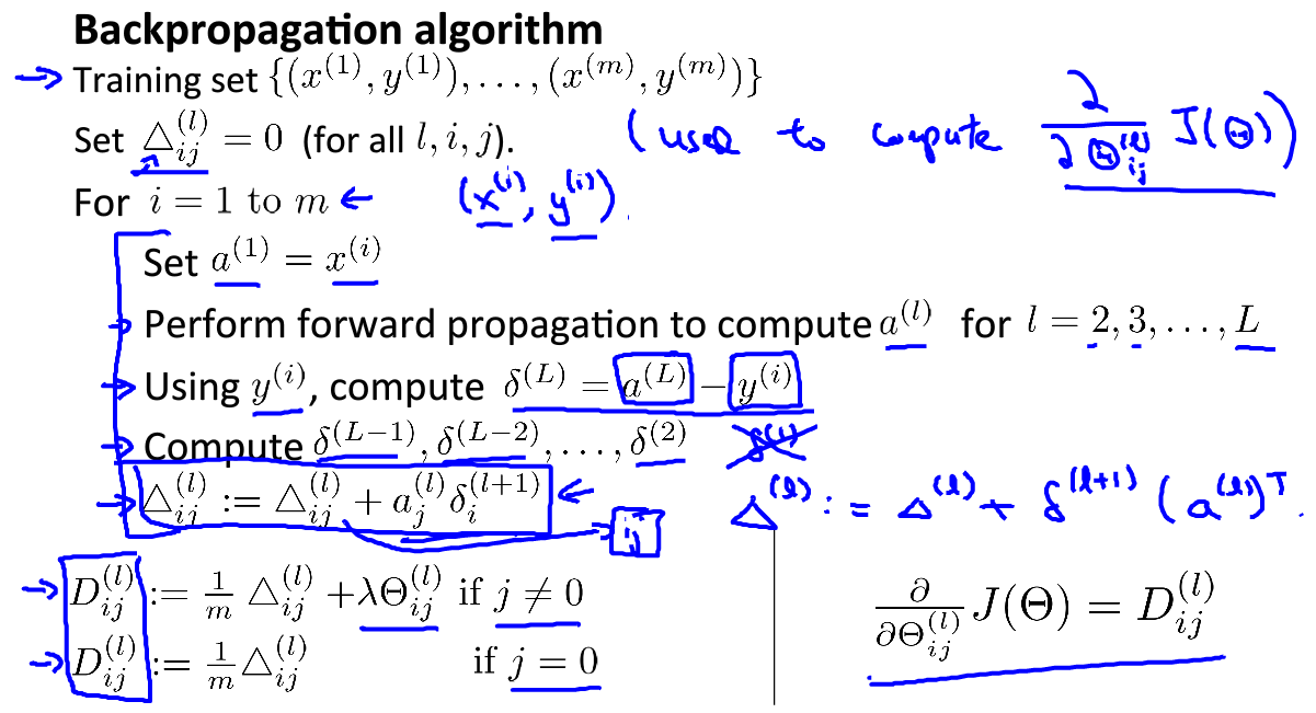
∂
∂
Θ
i
j
(
l
)
J
(
Θ
)
=
a
j
(
l
)
δ
i
(
l
+
1
)
\frac{\partial}{\partial\Theta_{ij}^{(l)}}J(\Theta)=a_j^{(l)}\delta_i^{(l+1)}
∂ Θ i j ( l ) ∂ J ( Θ ) = a j ( l ) δ i ( l + 1 )
{
(
x
(
1
)
,
y
(
1
)
)
,
…
,
(
x
(
m
)
,
y
(
m
)
)
}
\{(x^{(1)},y^{(1)}),\dots,(x^{(m)},y^{(m)})\}
{ ( x ( 1 ) , y ( 1 ) ) , … , ( x ( m ) , y ( m ) ) }
Δ
i
j
l
=
0
\Delta_{ij}^l=0
Δ i j l = 0
l
,
i
,
j
l,i,j
l , i , j
δ
j
(
l
)
=
∂
∂
z
j
(
l
)
c
o
s
t
(
i
)
\delta_j^{(l)}=\frac{\partial}{\partial z_{j}^{(l)}}cost(i)
δ j ( l ) = ∂ z j ( l ) ∂ c o s t ( i )
f
o
r
(
j
≥
0
)
for(j\geq0)
f o r ( j ≥ 0 )
c
o
s
t
(
i
)
=
y
(
i
)
log
(
h
θ
(
x
(
i
)
)
)
+
(
1
−
y
(
i
)
)
log
(
1
−
h
θ
(
x
(
i
)
)
)
cost(i)=y^{(i)}\log(h_\theta(x^{(i)}))+(1-y^{(i)})\log(1-h_\theta(x^{(i)}))
c o s t ( i ) = y ( i ) log ( h θ ( x ( i ) ) ) + ( 1 − y ( i ) ) log ( 1 − h θ ( x ( i ) ) )
δ
\delta
δ
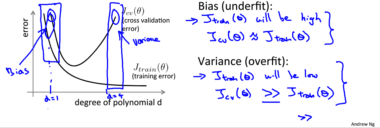
可以依据训练误差和测试误差来评估假设
h
θ
(
x
)
h_\theta(x)
h θ ( x )
θ
\theta
θ
m
i
n
J
(
θ
)
minJ(\theta)
m i n J ( θ ) linear regression :
J
t
r
a
i
n
(
θ
)
=
1
2
m
t
r
a
i
n
∑
i
=
1
m
t
r
a
i
n
(
h
θ
(
x
t
r
a
i
n
(
i
)
)
−
y
t
r
a
i
n
(
i
)
)
2
J_{train}(\theta)=\frac{1}{2m_{train}} \sum_{i=1}^{m_{train}}(h_\theta(x_{train}^{(i)})-y_{train}^{(i)})^2
J t r a i n ( θ ) = 2 m t r a i n 1 i = 1 ∑ m t r a i n ( h θ ( x t r a i n ( i ) ) − y t r a i n ( i ) ) 2
J
c
v
(
θ
)
=
1
2
m
c
v
∑
i
=
1
m
c
v
(
h
θ
(
x
c
v
(
i
)
)
−
y
c
v
(
i
)
)
2
J_{cv}(\theta)=\frac{1}{2m_{cv}} \sum_{i=1}^{m_{cv}}(h_\theta(x_{cv}^{(i)})-y_{cv}^{(i)})^2
J c v ( θ ) = 2 m c v 1 i = 1 ∑ m c v ( h θ ( x c v ( i ) ) − y c v ( i ) ) 2 logistic regression :
J
t
r
a
i
n
(
θ
)
=
−
1
m
t
r
a
i
n
∑
i
=
1
m
t
r
a
i
n
(
y
t
r
a
i
n
(
i
)
log
(
h
θ
(
x
t
r
a
i
n
(
i
)
)
)
+
(
1
−
y
t
r
a
i
n
(
i
)
)
log
(
1
−
h
θ
(
x
t
r
a
i
n
(
i
)
)
)
)
J_{train}(\theta)=-\frac{1}{m_{train}}\sum_{i=1}^{m_{train}}(y_{train}^{(i)}\log(h_\theta(x_{train}^{(i)}))+(1-y_{train}^{(i)})\log(1-h_\theta(x_{train}^{(i)})))
J t r a i n ( θ ) = − m t r a i n 1 i = 1 ∑ m t r a i n ( y t r a i n ( i ) log ( h θ ( x t r a i n ( i ) ) ) + ( 1 − y t r a i n ( i ) ) log ( 1 − h θ ( x t r a i n ( i ) ) ) )
J
c
v
(
θ
)
=
−
1
m
c
v
∑
i
=
1
m
c
v
(
y
c
v
(
i
)
log
(
h
θ
(
x
c
v
(
i
)
)
)
+
(
1
−
y
c
v
(
i
)
)
log
(
1
−
h
θ
(
x
c
v
(
i
)
)
)
)
J_{cv}(\theta)=-\frac{1}{m_{cv}}\sum_{i=1}^{m_{cv}}(y_{cv}^{(i)}\log(h_\theta(x_{cv}^{(i)}))+(1-y_{cv}^{(i)})\log(1-h_\theta(x_{cv}^{(i)})))
J c v ( θ ) = − m c v 1 i = 1 ∑ m c v ( y c v ( i ) log ( h θ ( x c v ( i ) ) ) + ( 1 − y c v ( i ) ) log ( 1 − h θ ( x c v ( i ) ) ) )
J
c
v
(
θ
)
J_{cv}(\theta)
J c v ( θ )
J
t
e
s
t
(
θ
)
J_{test}(\theta)
J t e s t ( θ )
e
r
r
o
r
=
{
1
,
if
y
i
=
1
,
h
θ
(
x
)
<
0.5
o
r
y
i
=
0
,
h
θ
(
x
)
≥
0.5
0
,
if
y
i
=
1
,
h
θ
(
x
)
≥
0.5
o
r
y
i
=
0
,
h
θ
(
x
)
<
0.5
error=\begin{cases} 1,\text{if $y_i=1,h_\theta(x)<0.5\ or\ y_i=0,h_\theta(x)\geq0.5$} \\ 0 ,\text{if $y_i=1,h_\theta(x)\geq0.5\ or\ y_i=0,h_\theta(x)<0.5$}\end{cases}
e r r o r = { 1 , if y i = 1 , h θ ( x ) < 0.5 or y i = 0 , h θ ( x ) ≥ 0.5 0 , if y i = 1 , h θ ( x ) ≥ 0.5 or y i = 0 , h θ ( x ) < 0.5
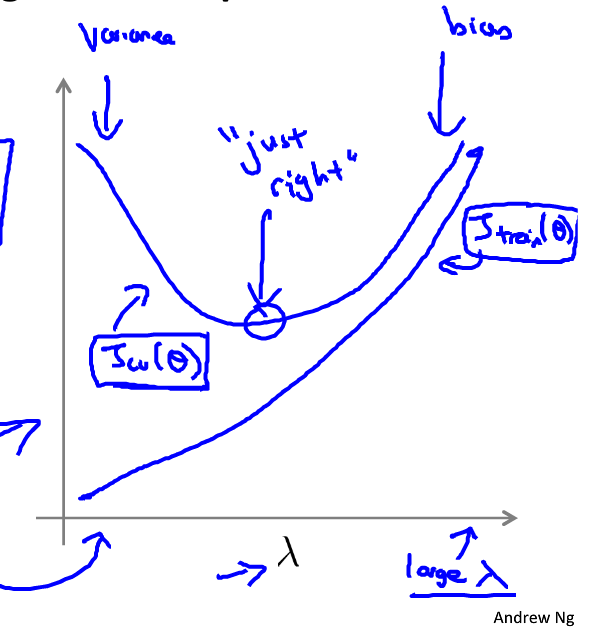
如图:
λ
\lambda
λ 较大 时,
θ
j
≈
0
\theta_j\approx0
θ j ≈ 0
θ
0
\theta_0
θ 0 欠拟合 ;
λ
\lambda
λ 较小 时,正则化项不起作用,模型会变得过拟合 。如图:
增加特征个数
增加多项式特征
降低
λ
\lambda
λ
对于高方差问题(过拟合):
增加训练样本
减少特征个数
增加
λ
\lambda
λ
对于神经网络来说,参数越少,越有可能欠拟合;参数越多,网络结构越复杂,越有可能过拟合,应该加入正则化项。