如何生成OBB（OrientedboundingBox）方向包围盒

版权声明：本文为博主原创文章，未经博主允许不得转载。需要转载请留言或发送邮件([email protected])，并注明出处。 https://blog.csdn.net/u013512448/article/details/52527237

一、包围盒简介：

          包围盒是一个简单的几何空间，里面包含着复杂形状的物体。为物体添加包围体的目的是快速的进行碰撞检测或者进行精确的碰撞检测之前进行过滤（即当包围体碰撞，才进行精确碰撞检测和处理）。包围体类型包括球体、轴对齐包围盒（AABB）、有向包围盒（OBB）、8-DOP以及凸壳。

包围盒广泛地应用于碰撞检测，比如射击、点击、相撞等，每一个物体都有自己的包围盒。因为包围盒一般为规则物体，因此用它来代替物体本身进行计算，会比直接用物体本身更加高效和简单。

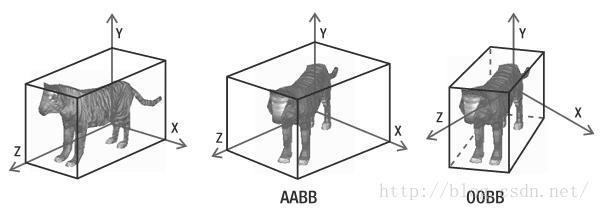
         目前广泛应用的是AABB和OBB包围盒，其中AABB包围盒更常见。因为它的生成方法很简单，因它与坐标轴是对齐的。但它也有不足，它不随物体旋转，可以看出当图中的老虎沿着Z轴方向站立时，AABB包围盒还和老虎比较贴合，但当老虎转了一个角度后，AABB包围盒便增加了较大的空隙，对于较精确的碰撞检测效果不太好。这时就需要OBB包围盒，它始终沿着物体的主成分方向生成最小的一个矩形包围盒，可以随物体旋转，可用于较精确的碰撞检测。

二、OBB包围盒生成思路：

OBB的生成思路简单来说就是根据物体表面的顶点，通过PCA（主成分分析）获得特征向量，即OBB的主轴。

主成分分析是一种通过正交变换，将一组可能相关的变量集合变换成一组线性不相关的变量集合，即主成分。

在这里就要引入协方差矩阵的概念，如果学过线性代数就会知道。协方差表示的使两个变量之间的线性相关程度。协方差越小则表示两个变量之间越独立，即线性相关性小。

通过协方差的计算公式，可以得到协方差矩阵。

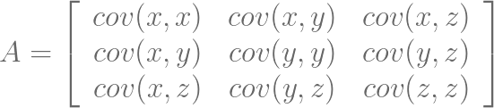
主对角线的元素表示变量的方差。主对角线的元素较大则表示强信号。非主对角线的元素表示变量之间的协方差。较大的非对角线元素表示数据的畸变。

为了减小畸变，可以重新定义变量间的线性组合，将协方差矩阵对角化。协方差矩阵的的元素是实数并且对称。

协方差矩阵的特征向量表示OBB包围盒的方向。大的特征值对应大的方差，所以应该让OBB包围盒沿着最大特征值对应的特征向量的方向。

例：

有如下一些点：

(3.7, 1.7), (4.1, 3.8), (4.7, 2.9), (5.2, 2.8), (6.0, 4.0), (6.3, 3.6), (9.7, 6.3), (10.0, 4.9), (11.0, 3.6), (12.5, 6.4)

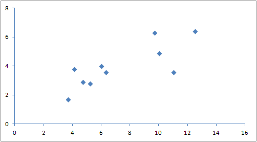
计算得到协方差矩阵：

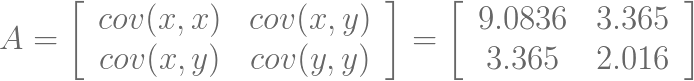
对角化协方差矩阵：

于是可以得到特征向量，也就是OBB的坐标轴：

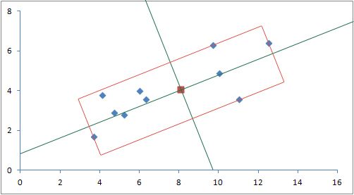
再计算得到OBB的中心点（8.10，4.05)，长宽的半长度分别为4.96 和1.49。即可一画出二维平面若干点生成的OBB包围盒。

关于讲解详细地可以查阅协方差矩阵和PCA分析的相关文章。我参考了如下两篇：

1、OBB generate via PCA：  https://hewjunwei.wordpress.com/2013/01/26/obb-generation-via-principal-component-analysis/

2、PCA的数学原理：    http://blog.csdn.net/xiaojidan2011/article/details/11595869

三、代码实现：

思路：

首先计算出协方差矩阵，用雅可比迭代法求出特征向量，再进行施密特正交化。

1、计算协方差矩阵

<span style="font-size:14px;">public Matrix3 computeCovarianceMatrix(Vector3[] pVertices,int numVertices) throws CloneNotSupportedException{
		Matrix3 covariance=new Matrix3();	
		Vector3[] pVectors=new Vector3[numVertices];
		
		//Compute the average x,y,z
		Vector3 avg=new Vector3(0.0f,0.0f,0.0f);
		for(int i=0;i<numVertices;i++){
			pVectors[i]= (Vector3)pVertices[i].clone();
			avg.add(pVertices[i]);
		}
		avg.divide(numVertices);
		for(int i=0;i<numVertices;i++)
			pVectors[i].sub(avg);
		
		//Compute the covariance 
		for(int c=0;c<3;c++)
		{
			float data[]=new float[3];
			for(int r=c;r<3;r++)
			{
				covariance.setColRow(c, r, 0.0f);
				float acc=0.0f;
				//cov(X,Y)=E[(X-x)(Y-y)]
				for(int i=0;i<numVertices;i++)
				{
					data[0]=pVectors[i].x;
					data[1]=pVectors[i].y;
					data[2]=pVectors[i].z;
					acc+=data[c]*data[r];
				}
				
				acc/=numVertices;
				covariance.setColRow(c, r, acc);
				//symmetric
				covariance.setColRow(r, c, acc);
			}
			
		}
		return covariance;
		
	}</span>

2、雅可比迭代法求出特征向量：

	public void jacobiSolver(Matrix3 matrix,float[] eValue ,Vector3[] eVectors ){
		float eps1=(float)0.00001;
		float eps2=(float)0.00001;
		float eps3=(float)0.00001;
		
		System.out.println("----------the 1.e-5----------");
		System.out.println(eps1);
		
		float p,q,spq;
		float cosa = 0,sina=0;  //cos(alpha) and sin(alpha)
		float temp;
		float s1=0.0f;    //sums of squares of diagonal
		float s2;          //elements
		
		boolean flag=true;  //determine whether to iterate again
		int iteration=0;   //iteration counter
		
		Vector3 mik=new Vector3() ;//used for temporaty storage of m[i][k]
		float[] data=new float[3];
		Matrix3 t=new Matrix3();//To store the product of the rotation matrices.
		t=Matrix3.identity();
		do{
			
			iteration++;
			
			for(int i=0;i<2;i++)
			{
				for(int j=i+1;j<3;j++)
				{
					if(Math.abs(matrix.getColRow(j, i))<eps1)
						matrix.setColRow(j, i, 0.0f);
					else{
						q=Math.abs(matrix.getColRow(i, i)-matrix.getColRow(j, j));
						if(q>eps2){
							p=(2.0f*matrix.getColRow(j, i)*q)/(matrix.getColRow(i, i)-matrix.getColRow(j, j));
							spq=(float)Math.sqrt(p*p+q*q);
							cosa=(float)Math.sqrt((1.0f+q/spq)/2.0f);
							sina=p/(2.0f*cosa*spq);
						}
						else
							sina=cosa=INV_SQRT_TWO;
					
					for(int k=0;k<3;k++){
						temp=t.getColRow(i, k);
						t.setColRow(i, k, (temp*cosa+t.getColRow(j, k)*sina));
						t.setColRow(j, k, (temp*sina-t.getColRow(j, k)*cosa));
					}
					for(int k=i;k<3;k++)
					{
						if(k>j){
							temp=matrix.getColRow(k, i);
							matrix.setColRow(k, i, (cosa*temp+sina*matrix.getColRow(k, j)));
							matrix.setColRow(k, j, (sina*temp-cosa*matrix.getColRow(k, j)));
						}
						else
						{
							data[k]=matrix.getColRow(k, i);
							matrix.setColRow(k, i, (cosa*data[k]+sina*matrix.getColRow(j, k)));
							
							if(k==j)
								matrix.setColRow(k, j, (sina*data[k]-cosa*matrix.getColRow(k, j)));
						}
					}
					data[j]=sina*data[i]-cosa*data[j];
					
					for(int k=0;k<=j;k++)
					{
						if(k<=i)
						{
							temp=matrix.getColRow(i, k);
							matrix.setColRow(i, k, (cosa*temp+sina*matrix.getColRow(j, k)));
							matrix.setColRow(j, k, (sina*temp-cosa*matrix.getColRow(j, k)));
							
						}
						else
							matrix.setColRow(j, k, (sina*data[k]-cosa*matrix.getColRow(j, k)));
						
					}
					}
					}
			}
			s2=0.0f;
			for(int i=0;i<3;i++)
			{
				eValue[i]=matrix.getColRow(i, i);
				s2+=eValue[i]*eValue[i];
			}
			
			if(Math.abs(s2)<(float)1.e-5||Math.abs(1-s1/s2)<eps3)
				flag=false;
			else
				s1=s2;
		}while(flag);
		
		eVectors[0].x=t.data[0];
		eVectors[0].y=t.data[1];
		eVectors[0].z=t.data[2];
		eVectors[1].x=t.data[3];
		eVectors[1].y=t.data[4];
		eVectors[1].z=t.data[5];
		eVectors[2].x=t.data[6];
		eVectors[2].y=t.data[7];
		eVectors[2].z=t.data[8];
		
		System.out.println("----------------eVector without transform-----------");
		for(int i=0;i<3;i++)
			printVector(eVectors[i]);
		System.out.println();
		
		mik.x=data[0];
		mik.y=data[1];
		mik.z=data[2];
		Vector3 cross=new Vector3();
		Vector3.cross(cross, eVectors[0], eVectors[1]);
		if((Vector3.dot(cross, eVectors[2])<0.0f))
				eVectors[2].inverse();
		
	}

3、施密特正交化：

//Schmidt orthogonal
	public void schmidtOrthogonal(Vector3 v0,Vector3 v1,Vector3 v2){
		v0.normalize();
		System.out.println("------------v0 normalized--------------");
		printVector(v0);
		
		//v1-=(v1*v0)*v0;
		System.out.println("------------v1 dot v0--------------");
		System.out.println(v1.dot(v0));
		v1.sub(Vector3.multiply(v1.dot(v0),v0));
		v1.normalize();
		Vector3.cross(v2,v0, v1);
	}

4、计算半长度

将各点的（X，Y，Z）坐标投影到计算出的坐标轴上，position由累加所有点再求均值得到。求出center和半长度。

              <pre name="code" class="java">                float infinity=Float.MAX_VALUE;
		Vector3 minExtents =new Vector3(infinity,infinity,infinity);
		Vector3 maxExtents=new Vector3(-infinity,-infinity,-infinity);
		
		for(int index=0;index<numVertices;index++)
		{
			Vector3 vec=vertices[index];
			Vector3 displacement =Vector3.sub(vec, position);
			
			minExtents.x=min(minExtents.x, Vector3.dot(displacement, orientation.getRowVector(1)));
			minExtents.y=min(minExtents.y, Vector3.dot(displacement, orientation.getRowVector(2)));
			minExtents.z=min(minExtents.z, Vector3.dot(displacement, orientation.getRowVector(3)));
			
			maxExtents.x=max(maxExtents.x, Vector3.dot(displacement, orientation.getRowVector(1)));
			maxExtents.y=max(maxExtents.y, Vector3.dot(displacement, orientation.getRowVector(2)));
			maxExtents.z=max(maxExtents.z, Vector3.dot(displacement, orientation.getRowVector(3)));
			
		}
		//offset = (maxExtents-minExtents)/2.0f+minExtents 
		Vector3 offset=Vector3.sub(maxExtents, minExtents);
		offset.divide(2.0f);
		offset.add(minExtents);
		
		System.out.println("-----------the offset-------------");
		printVector(offset);

<span style="white-space:pre">		</span>//中心点
		position.add(orientation.getRowVector(1).multiply(offset.x));
		position.add(orientation.getRowVector(2).multiply(offset.y));
		position.add(orientation.getRowVector(3).multiply(offset.z));
		//半长度
		halfExtents.x=(maxExtents.x-minExtents.x)/2.0f;
		halfExtents.y=(maxExtents.y-minExtents.y)/2.0f;
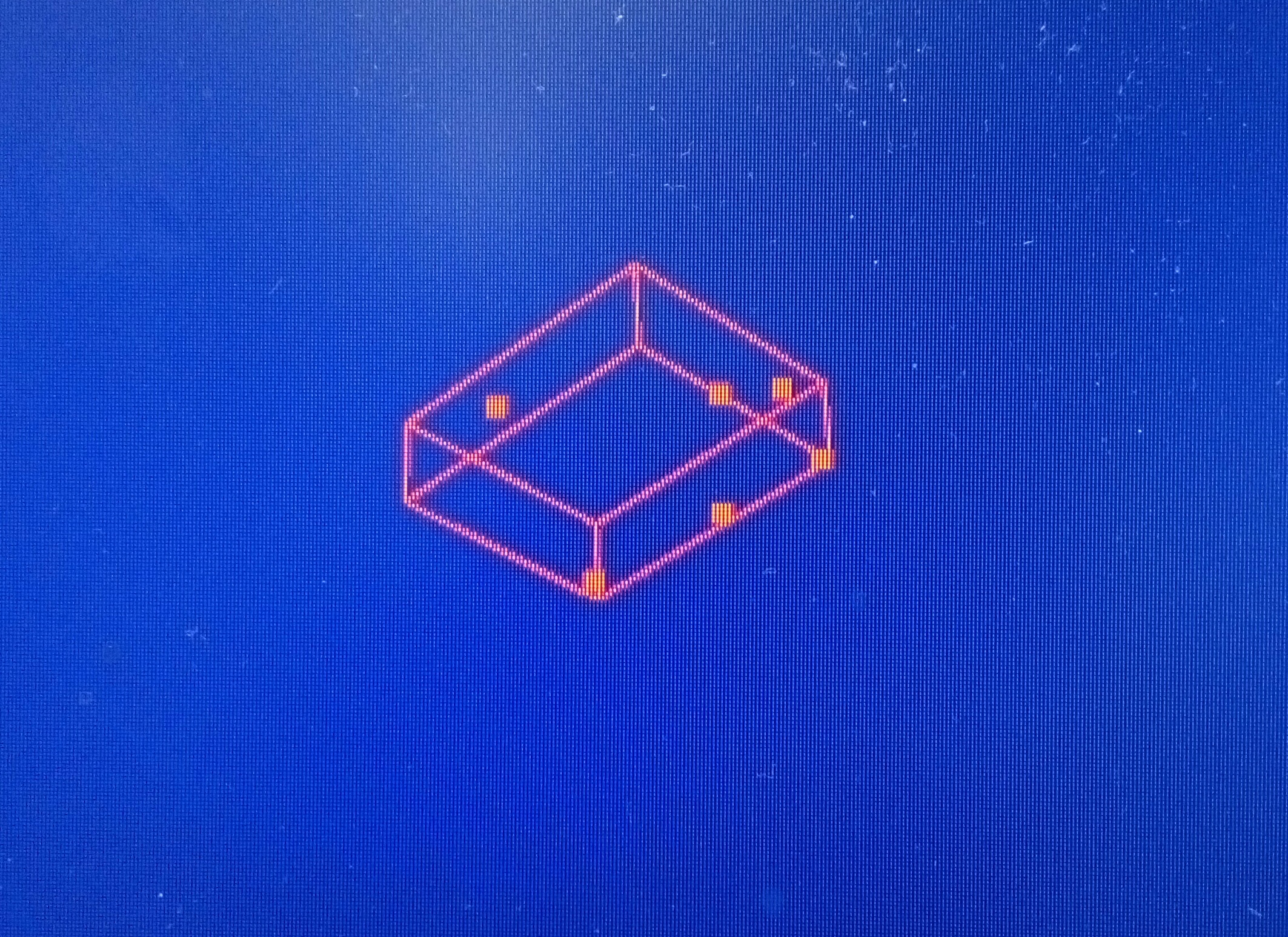
		halfExtents.z=(maxExtents.z-minExtents.z)/2.0f;

这是通过随机点生成的包围盒：