1. Problem:
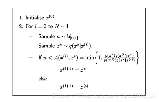
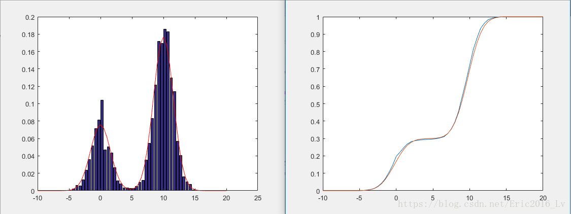
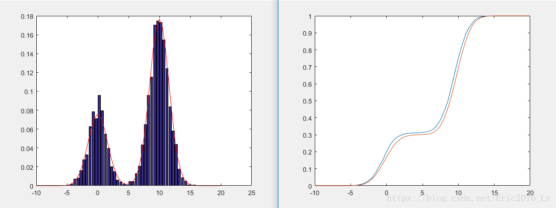
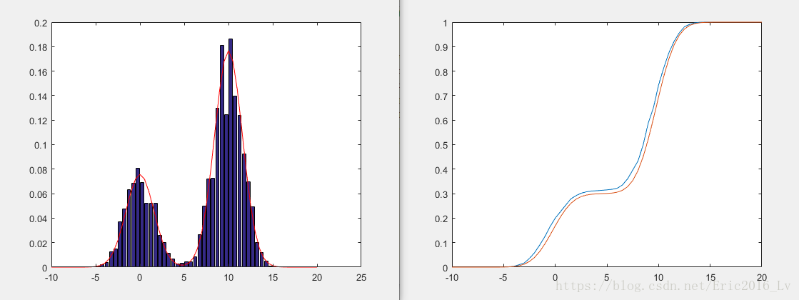
An MH step of invariant distribution and proposal distribution involves sampling a candidate value given the current value according to . The Markov chain then moves towards with acceptance probability , otherwise it remains at . The pseudo code is shown in the figure 1, while the following figures show the results of running the MHs algorithm with a Gaussian proposal distribution and a bimodal target distribution for 10000 iterations. As expected, the histogram of the samples approximates the target distribution.
2. Pseudo code:
3. MHs cases:
Case 1: General acceptance probability:
Acceptance probability:
Case 2: Metropolis algorithm:
Acceptance probability:
Case 3: Independent sampler:
Acceptance probability:
4. Matlab code:
% Metropolis(-Hastings) algorithm
% true (target) pdf is p(x) where we know it but can't sample data.
% proposal (sample) pdf is q(x*|x)=N(x,10) where we can sample.
%%
clc
clear;

X(1)=0;
N=1e4;
p = @(x) 0.3*exp(-0.2*x.^2) + 0.7*exp(-0.2*(x-10).^2);
dx=0.5; xx=-10:dx:20; fp=p(xx); plot(xx,fp) % plot the true p(x)
%% MH algorithm
sig=(10);
for i=1:N-1
    u=rand;
    x=X(i);
    xs=normrnd(x,sig); % new sample xs based on existing x from proposal pdf.
    pxs=p(xs);
    px=p(x);
    qxs=normpdf(xs,x,sig);
    qx=normpdf(x,xs,sig); % get p,q.
     if u<min(1,pxs*qx/(px*qxs))  % case 1: pesudo code
%     if u<min(1,pxs/(px))        % case 2: Metropolis algorithm
%     if u<min(1,pxs/qxs/(px/qx)) % case 3: independent sampler
        X(i+1)=xs;
    else
        X(i+1)=x;
    end
end
% compare pdf of the simulation result with true pdf.
N0=1;  close all;figure; %N/5;
nb=histc(X(N0+1:N),xx);
bar(xx+dx/2,nb/(N-N0)/dx); % plot samples.
A=sum(fp)*dx;
hold on; plot(xx,fp/A,'r') % compare.
% figure(2); plot(N0+1:N,X(N0+1:N)) % plot the traces of x.

% compare cdf with true cdf.
F1(1)=0;
F2(1)=0;
for i=2:length(xx)
  F1(i)=F1(i-1)+nb(i)/(N-N0);
  F2(i)=F2(i-1)+fp(i)*dx/A;
end

figure
plot(xx,[F1' F2'])
max(F1-F2) % this is the true possible measure of accuracy.
5. Results:
Result of Case 1:
Result of Case 2:
Result of Case 3:
References:
- An Introduction to MCMC for Machine Learning
- http://www2.mae.ufl.edu/haftka/vvuq/lectures/MCMC-Metropolis-practice.pptx