前言:本篇博文主要介绍神经网络(Neural network),介绍一下正则化用于神经网络防止过拟合,以及介绍多分类问题,然后通过Python代码实现相关模型。特别强调,其中大多理论知识来源于《统计学习方法_李航》和斯坦福课程翻译笔记以及Coursera机器学习课程。
本篇博文的理论知识都来自于吴大大的Coursera机器学习课程,人家讲的深入浅出,我就不一一赘述,只是简单概括一下以及记一下自己的见解。
1.神经网络模型
详细的神经网络模型,请参见我前面的博文介绍,其实还是强烈推荐这个斯坦福课程翻译笔记。
2.正则化防止过拟合
这里用逻辑回归为例,因为神经网络的最后一层(输出层)其实就可以看做逻辑回归。
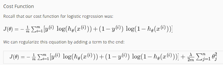
对比发现,就是在后面加了一坨平方的值,这个叫做“L2范式”。那么他的作用是什么呢?——就是“惩罚复杂的模型,倾向于小而简单的模型”——这其实是“方差与偏差”的一个权衡。
3.多分类问题
对于二分类问题(one vs one),我们的参数W=[w0,w1]是一维向量,代表一个分类器;那么对于多分类问题(n_classes = 4个类),我们采用(one vs rest),训练4个分类器,那W就是4个一维向量。如下,其中一列代表一个分类器。
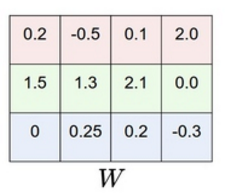
那么,相应的y也有变化,由原来的y=0——>y=[1,0,0,0]; y=1——>y=[0,1,0,0];y=2——>y=[0,0,1,0]
y=3——>y=[0,0,0,1]
4.BP传播算法
BP反向传播的原理,其实就是沿着表达式,根据链式法则,反向将梯度(gradient)进行传递。详情推荐反向传播笔记,这个应该是我看过最好的解释了(加个之一吧)。
5.代码实现
数据集还是原来的手写字体的识别。
#load the datasets
from sklearn.datasets import load_digits
import numpy as np
import matplotlib.pyplot as plt

digits = load_digits()
print digits.keys()
data = digits.data
target = digits.target

print data.shape
print target.shape
print data[15]
print "the images 15 is",target[15]
plt.gray()
plt.matshow(digits.images[15])
plt.show()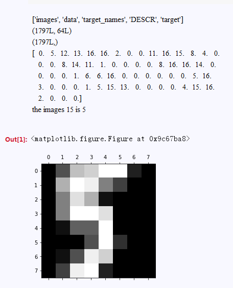
classes = ['0', '1', '2', '3', '4', '5', '6', '7', '8', '9']
num_classes = len(classes)
samples_per_class = 1
for y, cla in enumerate(classes):
    idxs = np.flatnonzero(target == y)
    idxs = np.random.choice(idxs, samples_per_class, replace=False)
    for i, idx in enumerate(idxs):
        plt_idx = i * num_classes + y + 1
        plt.subplot(samples_per_class, num_classes, plt_idx)
        plt.imshow(digits.images[idx].astype('uint8'))
        plt.axis('off')
        if i == 0:
            plt.title(cla)
plt.show()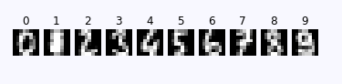
编写神经网络的类
#implement the neural network
def sigmoid(x):
    return 1/(1+np.exp(-x))

def dsigmoid(x):
    return x*(1-x)

class NeuralNetwork(object):
    def __init__(self,input_size,hidden_size,output_size):
        self.W1 = 0.01 * np.random.randn(input_size,hidden_size)#D*H
        self.b1 = np.zeros(hidden_size) #H
        self.W2 = 0.01 * np.random.randn(hidden_size,output_size)#H*C
        self.b2 = np.zeros(output_size)#C

    def loss(self,X,y,reg = 0.01):
        num_train, num_feature = X.shape
        #forward
        a1 = X  #input layer:N*D
        a2 = sigmoid(a1.dot(self.W1) + self.b1) #hidden layer:N*H
        a3 = sigmoid(a2.dot(self.W2) + self.b2) #output layer:N*C

        loss = - np.sum(y*np.log(a3) + (1-y)*np.log((1-a3)))/num_train
        loss += 0.5 * reg * (np.sum(self.W1*self.W1)+np.sum(self.W2*self.W2)) / num_train

        #backward
        error3 = a3 - y #N*C
        dW2 = a2.T.dot(error3) + reg * self.W2#(H*N)*(N*C)=H*C
        db2 = np.sum(error3,axis=0)

        error2 = error3.dot(self.W2.T)*dsigmoid(a2) #N*H
        dW1 = a1.T.dot(error2) + reg * self.W1     #(D*N)*(N*H) =D*H
        db1 = np.sum(error2,axis=0)

        dW1 /= num_train
        dW2 /= num_train
        db1 /= num_train
        db2 /= num_train

        return loss,dW1,dW2,db1,db2

    def train(self,X,y,y_train,X_val,y_val,learn_rate=0.01,num_iters = 10000):
        batch_size = 150
        num_train = X.shape[0]
        loss_list = []
        accuracy_train = []
        accuracy_val = []

        for i in xrange(num_iters):
            batch_index = np.random.choice(num_train,batch_size,replace=True)
            X_batch = X[batch_index]
            y_batch = y[batch_index]
            y_train_batch = y_train[batch_index]

            loss,dW1,dW2,db1,db2 = self.loss(X_batch,y_batch)
            loss_list.append(loss)

            #update the weight
            self.W1 += -learn_rate*dW1
            self.W2 += -learn_rate*dW2
            self.b1 += -learn_rate*db1
            self.b2 += -learn_rate*db2

            if i%500 == 0:
                print "i=%d,loss=%f" %(i,loss)
                #record the train accuracy and validation accuracy
                train_acc = np.mean(y_train_batch==self.predict(X_batch))
                val_acc = np.mean(y_val==self.predict(X_val))
                accuracy_train.append(train_acc)
                accuracy_val.append(val_acc)

        return loss_list,accuracy_train,accuracy_val

    def predict(self,X_test):
        a2 = sigmoid(X_test.dot(self.W1) + self.b1)
        a3 = sigmoid(a2.dot(self.W2) + self.b2)
        y_pred = np.argmax(a3,axis=1)
        return y_pred


    pass
划分数据集,进行训练一下,验证
from sklearn.model_selection import train_test_split
from sklearn.preprocessing import LabelBinarizer
X = data
y = target
#normalized
X_mean = np.mean(X,axis=0)
X -= X_mean

X_data,X_test,y_data,y_test = train_test_split(X,y,test_size=0.2)
#split the train and tne validation
X_train = X_data[0:1000]
y_train = y_data[0:1000]
X_val = X_data[1000:-1]
y_val = y_data[1000:-1]

print X_train.shape,X_val.shape,X_test.shape

y_train_label = LabelBinarizer().fit_transform(y_train)

classify = NeuralNetwork(X.shape[1],100,10)

print 'start'

loss_list,accuracy_train,accuracy_val = classify.train(X_train,y_train_label
                                                       ,y_train,X_val,y_val)


print 'end'
import matplotlib.pyplot as plt

plt.subplot(211)
plt.plot(loss_list)
plt.title('train loss')
plt.xlabel('iters')
plt.ylabel('loss')

plt.subplot(212)
plt.plot(accuracy_train,label = 'train_acc',color = 'red')
plt.plot(accuracy_val,label = 'val_acc', color = 'black')
plt.xlabel('iters')
plt.ylabel('accuracy')
plt.legend(loc = 'lower right')

plt.show()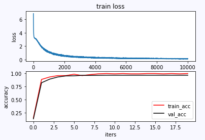
最后测试一下
y_pred = classify.predict(X_test)
accuracy = np.mean(y_pred == y_test)
print "the accuracy is ",accuracy
输出正确率:the accuracy is 0.977777777778